OCP Data Visualization#
import matplotlib
matplotlib.use('Agg')

import os
import numpy as np

import matplotlib.pyplot as plt
%matplotlib inline

params = {
   'axes.labelsize': 14,
   'font.size': 14,
   'font.family': ' DejaVu Sans',
   'legend.fontsize': 20,
   'xtick.labelsize': 20,
   'ytick.labelsize': 20,
   'axes.labelsize': 25,
   'axes.titlesize': 25,
   'text.usetex': False,
   'figure.figsize': [12, 12]
}
matplotlib.rcParams.update(params)


import ase.io
from ase.io.trajectory import Trajectory
from ase.io import extxyz
from ase.calculators.emt import EMT
from ase.build import fcc100, add_adsorbate, molecule
from ase.constraints import FixAtoms
from ase.optimize import LBFGS
from ase.visualize.plot import plot_atoms
from ase import Atoms
from IPython.display import Image
videos_dir = "videos/"
os.makedirs(videos_dir, exist_ok=True)

config = {
    "num_procs": 1,
    "fps": 30,
}
Understanding the data#
We use the Atomic Simulation Environment (ASE) to interact with our data. This notebook will provide you with some intuition on what the data looks like, how to visualize it, and the specific properties that are passed on to our models.
Generating sample data#
For simplicity, we generate sample data in the same format as the OC20 dataset. A toy relaxation (or trajectory) of propane (C3H8) on a copper (Cu) surface is used with a classical-like potential (EMT). Unlike DFT, EMT is extremely fast but limited in accuracy and applicability to certain elements, making it great for demos and tests. You are free to explore alternative systems below, however, you may skip the data construction and move on to “Reading a trajectory”.
###DATA GENERATION - FEEL FREE TO SKIP###

adslab = fcc100("Cu", size=(3, 3, 3))
adsorbate = molecule("C3H8")
add_adsorbate(adslab, adsorbate, 3, offset=(1, 1)) # adslab = adsorbate + slab

# tag all slab atoms below surface as 0, surface as 1, adsorbate as 2
tags = np.zeros(len(adslab))
tags[18:27] = 1
tags[27:] = 2

adslab.set_tags(tags)

# Fixed atoms are prevented from moving during a structure relaxation. We fix all slab atoms beneath the surface
cons= FixAtoms(indices=[atom.index for atom in adslab if (atom.tag == 0)])
adslab.set_constraint(cons)
adslab.center(vacuum=13.0, axis=2)
adslab.set_pbc(True)
adslab.set_calculator(EMT())

os.makedirs('data', exist_ok=True)

# Define structure optimizer - LBFGS. Run for 100 steps, or if the max force on all atoms (fmax) is below 0 ev/A.
# fmax is typically set to 0.01-0.05 eV/A, for this demo however we run for the full 100 steps.

dyn = LBFGS(adslab, trajectory="data/toy_c3h8_relax.traj")
dyn.run(fmax=0, steps=100)

traj = ase.io.read("data/toy_c3h8_relax.traj", ":")

# convert traj format to extxyz format (used by OC20 dataset)
columns = (['symbols','positions', 'move_mask', 'tags', 'forces'])
with open('data/toy_c3h8_relax.extxyz','w') as f:
    extxyz.write_xyz(f, traj, columns=columns)

os.system("rm data/toy_c3h8_relax.traj")
       Step     Time          Energy          fmax
LBFGS:    0 19:52:14       15.804700        6.776430
LBFGS: 1 19:52:14 12.190607 4.323222
LBFGS: 2 19:52:14 10.240169 2.265527
LBFGS: 3 19:52:14 9.779223 0.937247
LBFGS: 4 19:52:14 9.671525 0.770173
LBFGS: 5 19:52:14 9.574461 0.663540
LBFGS: 6 19:52:14 9.537502 0.571800
LBFGS: 7 19:52:14 9.516673 0.446620
LBFGS: 8 19:52:14 9.481330 0.461143
LBFGS: 9 19:52:14 9.462255 0.293081
LBFGS: 10 19:52:14 9.448937 0.249010
LBFGS: 11 19:52:14 9.433813 0.237051
LBFGS: 12 19:52:14 9.418884 0.260245
LBFGS: 13 19:52:14 9.409649 0.253162
LBFGS: 14 19:52:14 9.404838 0.162398
LBFGS: 15 19:52:14 9.401753 0.182298
LBFGS: 16 19:52:14 9.397314 0.259163
/tmp/ipykernel_5286/2542206394.py:19: FutureWarning: Please use atoms.calc = calc
  adslab.set_calculator(EMT())
LBFGS: 17 19:52:14 9.387947 0.345022
LBFGS: 18 19:52:14 9.370825 0.407041
LBFGS: 19 19:52:14 9.342222 0.433340
LBFGS: 20 19:52:14 9.286822 0.500200
LBFGS: 21 19:52:14 9.249910 0.524052
LBFGS: 22 19:52:14 9.187179 0.511994
LBFGS: 23 19:52:14 9.124811 0.571796
LBFGS: 24 19:52:14 9.066185 0.540934
LBFGS: 25 19:52:14 9.000116 1.079833
LBFGS: 26 19:52:14 8.893632 0.752759
LBFGS: 27 19:52:14 8.845939 0.332051
LBFGS: 28 19:52:14 8.815173 0.251242
LBFGS: 29 19:52:14 8.808721 0.214337
LBFGS: 30 19:52:14 8.794643 0.154611
LBFGS: 31 19:52:14 8.789162 0.201404
LBFGS: 32 19:52:14 8.782320 0.175517
LBFGS: 33 19:52:14 8.780394 0.103718
LBFGS: 34 19:52:14 8.778410 0.107611
LBFGS: 35 19:52:14 8.775079 0.179747
LBFGS: 36 19:52:14 8.766987 0.333401
LBFGS: 37 19:52:14 8.750249 0.530715
LBFGS: 38 19:52:14 8.725928 0.685116
LBFGS: 39 19:52:14 8.702312 0.582260
LBFGS: 40 19:52:14 8.661515 0.399625
LBFGS: 41 19:52:14 8.643432 0.558474
LBFGS: 42 19:52:14 8.621201 0.367288
LBFGS: 43 19:52:14 8.614414 0.139424
LBFGS: 44 19:52:14 8.610785 0.137160
LBFGS: 45 19:52:14 8.608134 0.146375
LBFGS: 46 19:52:14 8.604928 0.119648
LBFGS: 47 19:52:14 8.599151 0.135424
LBFGS: 48 19:52:14 8.594063 0.147913
LBFGS: 49 19:52:15 8.589493 0.153840
LBFGS: 50 19:52:15 8.587274 0.088460
LBFGS: 51 19:52:15 8.584633 0.093750
LBFGS: 52 19:52:15 8.580239 0.140870
LBFGS: 53 19:52:15 8.572938 0.254272
LBFGS: 54 19:52:15 8.563343 0.291885
LBFGS: 55 19:52:15 8.554117 0.196557
LBFGS: 56 19:52:15 8.547597 0.129064
LBFGS: 57 19:52:15 8.542086 0.128020
LBFGS: 58 19:52:15 8.535432 0.098202
LBFGS: 59 19:52:15 8.533622 0.127672
LBFGS: 60 19:52:15 8.527487 0.116729
LBFGS: 61 19:52:15 8.523863 0.121762
LBFGS: 62 19:52:15 8.519229 0.130541
LBFGS: 63 19:52:15 8.515424 0.101902
LBFGS: 64 19:52:15 8.511240 0.212223
LBFGS: 65 19:52:15 8.507967 0.266593
LBFGS: 66 19:52:15 8.503903 0.237734
LBFGS: 67 19:52:15 8.497575 0.162253
LBFGS: 68 19:52:15 8.485434 0.202203
LBFGS: 69 19:52:15 8.466738 0.215895
LBFGS: 70 19:52:15 8.467607 0.334764
LBFGS: 71 19:52:15 8.454037 0.106310
LBFGS: 72 19:52:15 8.448980 0.119721
LBFGS: 73 19:52:15 8.446550 0.099221
LBFGS: 74 19:52:15 8.444705 0.056244
LBFGS: 75 19:52:15 8.443403 0.038831
LBFGS: 76 19:52:15 8.442646 0.054772
LBFGS: 77 19:52:15 8.442114 0.061370
LBFGS: 78 19:52:15 8.440960 0.058800
LBFGS: 79 19:52:15 8.439820 0.048198
LBFGS: 80 19:52:15 8.438600 0.051251
LBFGS: 81 19:52:15 8.437429 0.054130
LBFGS: 82 19:52:15 8.435695 0.067234
LBFGS: 83 19:52:15 8.431957 0.085678
LBFGS: 84 19:52:15 8.423485 0.133240
LBFGS: 85 19:52:15 8.413846 0.207812
LBFGS: 86 19:52:15 8.404849 0.178747
LBFGS: 87 19:52:15 8.385339 0.169017
LBFGS: 88 19:52:15 8.386849 0.187645
LBFGS: 89 19:52:15 8.371078 0.118124
LBFGS: 90 19:52:15 8.368801 0.094222
LBFGS: 91 19:52:15 8.366226 0.066960
LBFGS: 92 19:52:15 8.361680 0.054964
LBFGS: 93 19:52:15 8.360631 0.047342
LBFGS: 94 19:52:15 8.359692 0.024179
LBFGS: 95 19:52:15 8.359361 0.015549
LBFGS: 96 19:52:15 8.359163 0.014284
LBFGS: 97 19:52:15 8.359102 0.015615
LBFGS: 98 19:52:15 8.359048 0.015492
LBFGS: 99 19:52:15 8.358986 0.014214
LBFGS: 100 19:52:15 8.358921 0.013159
/opt/hostedtoolcache/Python/3.12.8/x64/lib/python3.12/site-packages/ase/io/extxyz.py:311: UserWarning: Skipping unhashable information adsorbate_info
  warnings.warn('Skipping unhashable information '
0
Reading a trajectory#
identifier = "toy_c3h8_relax.extxyz"
traj = ase.io.read("data/%s" % identifier, index=":")
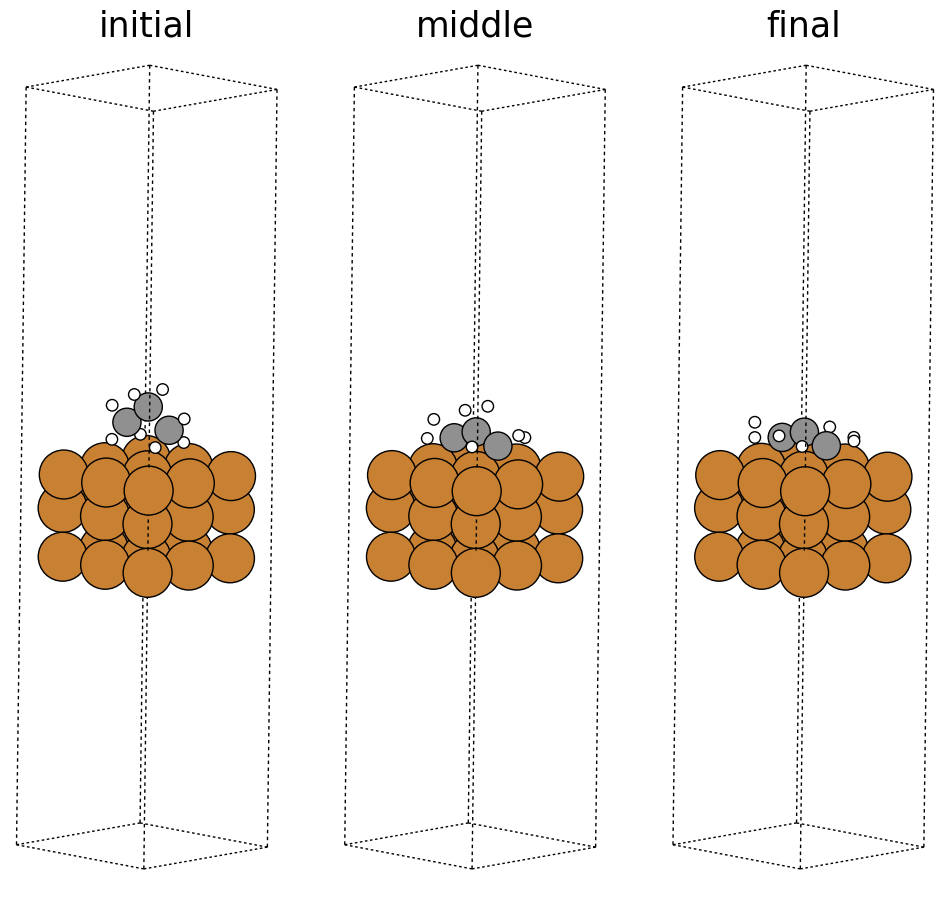
Viewing a trajectory#
fig, ax = plt.subplots(1, 3)
labels = ['initial', 'middle', 'final']
for i in range(3):
    ax[i].axis('off')
    ax[i].set_title(labels[i])
ase.visualize.plot.plot_atoms(traj[0], ax[0], radii=0.8, rotation=("-75x, 45y, 10z"))
ase.visualize.plot.plot_atoms(traj[50], ax[1], radii=0.8, rotation=("-75x, 45y, 10z"))
ase.visualize.plot.plot_atoms(traj[-1], ax[2], radii=0.8, rotation=("-75x, 45y, 10z"))
<Axes: title={'center': 'final'}>
Saving a trajectory video#
More visualization resources can be found here: https://wiki.fysik.dtu.dk/ase/ase/visualize/visualize.html.
identifier = "toy_c3h8_relax.extxyz"
traj = ase.io.read("data/%s" % identifier, index=":")

ase.io.write(os.path.join(videos_dir, identifier + ".gif"),
             traj,
             interval=1,
             rotation=("-75x, 45y, 10z"))
plt.close()
Image(open(os.path.join(videos_dir, identifier + ".gif"),'rb').read())
MovieWriter ffmpeg unavailable; using Pillow instead.
Data contents#
Here we take a closer look at what information is contained within these trajectories.
i_structure = traj[0]
i_structure
Atoms(symbols='Cu27C3H8', pbc=True, cell=[7.65796644025031, 7.65796644025031, 33.266996999999996], tags=..., constraint=FixAtoms(indices=[0, 1, 2, 3, 4, 5, 6, 7, 8, 9, 10, 11, 12, 13, 14, 15, 16, 17]), calculator=SinglePointCalculator(...))
Atomic numbers#
numbers = i_structure.get_atomic_numbers()
print(numbers)
[29 29 29 29 29 29 29 29 29 29 29 29 29 29 29 29 29 29 29 29 29 29 29 29
 29 29 29  6  6  6  1  1  1  1  1  1  1  1]
Atomic symbols#
symbols = np.array(i_structure.get_chemical_symbols())
print(symbols)
['Cu' 'Cu' 'Cu' 'Cu' 'Cu' 'Cu' 'Cu' 'Cu' 'Cu' 'Cu' 'Cu' 'Cu' 'Cu' 'Cu'
 'Cu' 'Cu' 'Cu' 'Cu' 'Cu' 'Cu' 'Cu' 'Cu' 'Cu' 'Cu' 'Cu' 'Cu' 'Cu' 'C' 'C'
 'C' 'H' 'H' 'H' 'H' 'H' 'H' 'H' 'H']
Unit cell#
The unit cell is the volume containing our system of interest. Express as a 3x3 array representing the directional vectors that make up the volume. Illustrated as the dashed box in the above visuals.
cell = np.array(i_structure.cell)
print(cell)
[[ 7.65796644  0.          0.        ]
 [ 0.          7.65796644  0.        ]
 [ 0.          0.         33.266997  ]]
Periodic boundary conditions (PBC)#
x,y,z boolean representing whether a unit cell repeats in the corresponding directions. The OC20 dataset sets this to [True, True, True], with a large enough vacuum layer above the surface such that a unit cell does not see itself in the z direction.
pbc = i_structure.pbc
print(pbc)
[ True True True]
Fixed atoms constraint#
In reality, surfaces contain many, many more atoms beneath what we’ve illustrated as the surface. At an infinite depth, these subsurface atoms would look just like the bulk structure. We approximate a true surface by fixing the subsurface atoms into their “bulk” locations. This ensures that they cannot move at the “bottom” of the surface. If they could, this would throw off our calculations. Consistent with the above, we fix all atoms with tags=0, and denote them as “fixed”. All other atoms are considered “free”.
cons = i_structure.constraints[0]
print(cons, '\n')

# indices of fixed atoms
indices = cons.index
print(indices, '\n')

# fixed atoms correspond to tags = 0
print(tags[indices])
FixAtoms(indices=[0, 1, 2, 3, 4, 5, 6, 7, 8, 9, 10, 11, 12, 13, 14, 15, 16, 17])

[ 0  1  2  3  4  5  6  7  8  9 10 11 12 13 14 15 16 17]

[0 0 0 0 0 0 0 0 0 0 0 0 0 0 0 0 0 0]
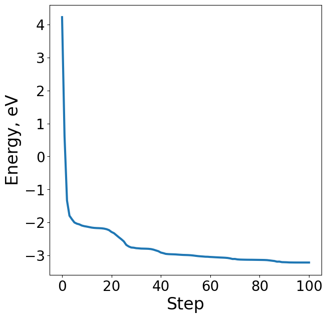
Energy#
The energy of the system is one of the properties of interest in the OC20 dataset. It’s important to note that absolute energies provide little value to researchers and must be referenced properly to be useful. The OC20 dataset references all it’s energies to the bare slab + gas references to arrive at adsorption energies. Adsorption energies are important in studying catalysts and their corresponding reaction rates. In addition to the structure realxations of the OC20 dataset, bare slab and gas (N2, H2, H2O, CO) relaxations were carried out with DFT in order to calculate adsorption energies.
final_structure = traj[-1]
relaxed_energy = final_structure.get_potential_energy()
print(f'Relaxed absolute energy = {relaxed_energy} eV')

# Corresponding raw slab used in original adslab (adsorbate+slab) system.
raw_slab = fcc100("Cu", size=(3, 3, 3))
raw_slab.set_calculator(EMT())
raw_slab_energy = raw_slab.get_potential_energy()
print(f'Raw slab energy = {raw_slab_energy} eV')


adsorbate = Atoms("C3H8").get_chemical_symbols()
# For clarity, we define arbitrary gas reference energies here.
# A more detailed discussion of these calculations can be found in the corresponding paper's SI.
gas_reference_energies = {'H': .3, 'O': .45, 'C': .35, 'N': .50}

adsorbate_reference_energy = 0
for ads in adsorbate:
    adsorbate_reference_energy += gas_reference_energies[ads]

print(f'Adsorbte reference energy = {adsorbate_reference_energy} eV\n')

adsorption_energy = relaxed_energy - raw_slab_energy - adsorbate_reference_energy
print(f'Adsorption energy: {adsorption_energy} eV')
Relaxed absolute energy = 8.358921451410891 eV
Raw slab energy = 8.127167122749576 eV
Adsorbte reference energy = 3.4499999999999993 eV

Adsorption energy: -3.2182456713386838 eV
/tmp/ipykernel_5286/1528962.py:7: FutureWarning: Please use atoms.calc = calc
  raw_slab.set_calculator(EMT())
# Plot energy profile of toy trajectory
energies = [image.get_potential_energy() - raw_slab_energy - adsorbate_reference_energy for image in traj]

plt.figure(figsize=(7, 7))
plt.plot(range(len(energies)), energies, lw=3)
plt.xlabel("Step", fontsize=24)
plt.ylabel("Energy, eV", fontsize=24)
Text(0, 0.5, 'Energy, eV')
Forces#
Forces are another important property of the OC20 dataset. Unlike datasets like QM9 which contain only ground state properties, the OC20 dataset contains per-atom forces necessary to carry out atomistic simulations. Physically, forces are the negative gradient of energy w.r.t atomic positions: \(F = -\frac{dE}{dx}\). Maintaining this energy-force consistency is important for models that seek to make predictions on both.
The “apply_constraint” argument controls whether to apply system constraints to the forces. In the OC20 dataset, this controls whether to return forces for fixed atoms (apply_constraint=False) or return 0s (apply_constraint=True).
# Returning forces for all atoms - regardless of whether "fixed" or "free"
i_structure.get_forces(apply_constraint=False)
array([[-1.07900000e-05, -3.80000000e-06,  1.13560540e-01],
       [ 0.00000000e+00, -4.29200000e-05,  1.13302410e-01],
       [ 1.07900000e-05, -3.80000000e-06,  1.13560540e-01],
       [-1.84600000e-05,  0.00000000e+00,  1.13543430e-01],
       [ 0.00000000e+00,  0.00000000e+00,  1.13047800e-01],
       [ 1.84600000e-05, -0.00000000e+00,  1.13543430e-01],
       [-1.07900000e-05,  3.80000000e-06,  1.13560540e-01],
       [-0.00000000e+00,  4.29200000e-05,  1.13302410e-01],
       [ 1.07900000e-05,  3.80000000e-06,  1.13560540e-01],
       [-1.10430500e-02, -2.53094000e-03, -4.84573700e-02],
       [ 1.10430500e-02, -2.53094000e-03, -4.84573700e-02],
       [-0.00000000e+00, -2.20890000e-04, -2.07827000e-03],
       [-1.10430500e-02,  2.53094000e-03, -4.84573700e-02],
       [ 1.10430500e-02,  2.53094000e-03, -4.84573700e-02],
       [-0.00000000e+00,  2.20890000e-04, -2.07827000e-03],
       [-3.49808000e-03, -0.00000000e+00, -7.85544000e-03],
       [ 3.49808000e-03, -0.00000000e+00, -7.85544000e-03],
       [-0.00000000e+00, -0.00000000e+00, -5.97640000e-04],
       [-3.18144370e-01, -2.36420450e-01, -3.97089230e-01],
       [ 0.00000000e+00, -2.18895316e+00, -2.74768262e+00],
       [ 3.18144370e-01, -2.36420450e-01, -3.97089230e-01],
       [-5.65980520e-01,  0.00000000e+00, -6.16046990e-01],
       [ 0.00000000e+00, -0.00000000e+00, -4.47152822e+00],
       [ 5.65980520e-01,  0.00000000e+00, -6.16046990e-01],
       [-3.18144370e-01,  2.36420450e-01, -3.97089230e-01],
       [-0.00000000e+00,  2.18895316e+00, -2.74768262e+00],
       [ 3.18144370e-01,  2.36420450e-01, -3.97089230e-01],
       [-0.00000000e+00,  0.00000000e+00, -3.96835355e+00],
       [-0.00000000e+00, -3.64190926e+00,  5.71458646e+00],
       [-0.00000000e+00,  3.64190926e+00,  5.71458646e+00],
       [-2.18178516e+00,  0.00000000e+00,  1.67589182e+00],
       [ 2.18178516e+00,  0.00000000e+00,  1.67589182e+00],
       [ 0.00000000e+00,  2.46333681e+00,  1.78299828e+00],
       [ 0.00000000e+00, -2.46333681e+00,  1.78299828e+00],
       [ 6.18714050e+00,  2.26336330e-01, -5.99485570e-01],
       [-6.18714050e+00,  2.26336330e-01, -5.99485570e-01],
       [-6.18714050e+00, -2.26336330e-01, -5.99485570e-01],
       [ 6.18714050e+00, -2.26336330e-01, -5.99485570e-01]])
# Applying the fixed atoms constraint to the forces
i_structure.get_forces(apply_constraint=True)
array([[ 0.        ,  0.        ,  0.        ],
       [ 0.        ,  0.        ,  0.        ],
       [ 0.        ,  0.        ,  0.        ],
       [ 0.        ,  0.        ,  0.        ],
       [ 0.        ,  0.        ,  0.        ],
       [ 0.        ,  0.        ,  0.        ],
       [ 0.        ,  0.        ,  0.        ],
       [ 0.        ,  0.        ,  0.        ],
       [ 0.        ,  0.        ,  0.        ],
       [ 0.        ,  0.        ,  0.        ],
       [ 0.        ,  0.        ,  0.        ],
       [ 0.        ,  0.        ,  0.        ],
       [ 0.        ,  0.        ,  0.        ],
       [ 0.        ,  0.        ,  0.        ],
       [ 0.        ,  0.        ,  0.        ],
       [ 0.        ,  0.        ,  0.        ],
       [ 0.        ,  0.        ,  0.        ],
       [ 0.        ,  0.        ,  0.        ],
       [-0.31814437, -0.23642045, -0.39708923],
       [ 0.        , -2.18895316, -2.74768262],
       [ 0.31814437, -0.23642045, -0.39708923],
       [-0.56598052,  0.        , -0.61604699],
       [ 0.        , -0.        , -4.47152822],
       [ 0.56598052,  0.        , -0.61604699],
       [-0.31814437,  0.23642045, -0.39708923],
       [-0.        ,  2.18895316, -2.74768262],
       [ 0.31814437,  0.23642045, -0.39708923],
       [-0.        ,  0.        , -3.96835355],
       [-0.        , -3.64190926,  5.71458646],
       [-0.        ,  3.64190926,  5.71458646],
       [-2.18178516,  0.        ,  1.67589182],
       [ 2.18178516,  0.        ,  1.67589182],
       [ 0.        ,  2.46333681,  1.78299828],
       [ 0.        , -2.46333681,  1.78299828],
       [ 6.1871405 ,  0.22633633, -0.59948557],
       [-6.1871405 ,  0.22633633, -0.59948557],
       [-6.1871405 , -0.22633633, -0.59948557],
       [ 6.1871405 , -0.22633633, -0.59948557]])
Resources#
More helpful resources, tutorials, and documentation can be found at ASE’s webpage: https://wiki.fysik.dtu.dk/ase/index.html. We point to specific pages that may be of interest:
Interacting with Atoms Object: https://wiki.fysik.dtu.dk/ase/ase/atoms.html
Visualization: https://wiki.fysik.dtu.dk/ase/ase/visualize/visualize.html
Structure optimization: https://wiki.fysik.dtu.dk/ase/ase/optimize.html
Tutorials: https://wiki.fysik.dtu.dk/ase/tutorials/tutorials.html