Using OCP to enumerate adsorbates on alloy catalyst surfaces#
In the previous example, we constructed slab models of adsorbates on desired sites. Here we leverage code to automate this process. The goal in this section is to generate candidate structures, compute energetics, and then filter out the most relevant ones.
from fairchem.core.common.relaxation.ase_utils import OCPCalculator
import ase.io
from ase.optimize import BFGS
import sys
from scipy.stats import linregress
import pickle
import matplotlib.pyplot as plt
import time

from fairchem.data.oc.core import Adsorbate, AdsorbateSlabConfig, Bulk, Slab
import os
from glob import glob
import pandas as pd
from fairchem.data.oc.utils import DetectTrajAnomaly

# Set random seed to ensure adsorbate enumeration yields a valid candidate
# If using a larger number of random samples this wouldn't be necessary
import numpy as np
np.random.seed(22)
from fairchem.core.models.model_registry import model_name_to_local_file

checkpoint_path = model_name_to_local_file('EquiformerV2-31M-S2EF-OC20-All+MD', local_cache='/tmp/fairchem_checkpoints/')
checkpoint_path
'/tmp/fairchem_checkpoints/eq2_31M_ec4_allmd.pt'
Introduction#
We will reproduce Fig 6b from the following paper: Zhou, Jing, et al. “Enhanced Catalytic Activity of Bimetallic Ordered Catalysts for Nitrogen Reduction Reaction by Perturbation of Scaling Relations.” ACS Catalysis 134 (2023): 2190-2201 (https://doi.org/10.1021/acscatal.2c05877).
The gist of this figure is a correlation between H* and NNH* adsorbates across many different alloy surfaces. Then, they identify a dividing line between these that separates surfaces known for HER and those known for NRR.
To do this, we will enumerate adsorbate-slab configurations and run ML relaxations on them to find the lowest energy configuration. We will assess parity between the model predicted values and those reported in the paper. Finally we will make the figure and assess separability of the NRR favored and HER favored domains.
Enumerate the adsorbate-slab configurations to run relaxations on#
Be sure to set the path in fairchem/data/oc/configs/paths.py to point to the correct place or pass the paths as an argument. The database pickles can be found in fairchem/data/oc/databases/pkls (some pkl files are only downloaded by running the command python src/fairchem/core/scripts/download_large_files.py oc from the root of the fairchem repo). We will show one explicitly here as an example and then run all of them in an automated fashion for brevity.
import fairchem.data.oc
from pathlib import Path
db = Path(fairchem.data.oc.__file__).parent / Path('databases/pkls/adsorbates.pkl')
db
PosixPath('/home/runner/work/fairchem/fairchem/src/fairchem/data/oc/databases/pkls/adsorbates.pkl')
Work out a single example#
We load one bulk id, create a bulk reference structure from it, then generate the surfaces we want to compute.
bulk_src_id = "oqmd-343039"
adsorbate_smiles_nnh = "*N*NH"
adsorbate_smiles_h = "*H"

bulk = Bulk(bulk_src_id_from_db = bulk_src_id, bulk_db_path="NRR_example_bulks.pkl")
adsorbate_H = Adsorbate(adsorbate_smiles_from_db = adsorbate_smiles_h, adsorbate_db_path=db)
adsorbate_NNH = Adsorbate(adsorbate_smiles_from_db = adsorbate_smiles_nnh, adsorbate_db_path=db)
slab = Slab.from_bulk_get_specific_millers(bulk= bulk, specific_millers = (1, 1, 1))
slab
[Slab: (Ag36Pd12, (1, 1, 1), 0.16666666666666669, True)]
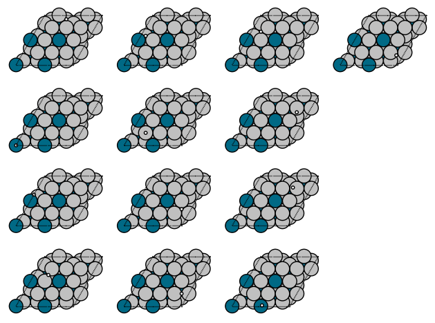
We now need to generate potential placements. We use two kinds of guesses, a heuristic and a random approach. This cell generates 13 potential adsorption geometries.
# Perform heuristic placements
heuristic_adslabs = AdsorbateSlabConfig(slab[0], adsorbate_H, mode="heuristic")

# Perform random placements
# (for AdsorbML we use `num_sites = 100` but we will use 4 for brevity here)
random_adslabs = AdsorbateSlabConfig(slab[0], adsorbate_H, mode="random_site_heuristic_placement", num_sites=4)

adslabs = [*heuristic_adslabs.atoms_list, *random_adslabs.atoms_list]
len(adslabs)
13
Let’s see what we are looking at. It is a little tricky to see the tiny H atom in these figures, but with some inspection you can see there are ontop, bridge, and hollow sites in different places. This is not an exhaustive search; you can increase the number of random placements to check more possibilities. The main idea here is to increase the probability you find the most relevant sites.
import matplotlib.pyplot as plt
from ase.visualize.plot import plot_atoms

fig, axs = plt.subplots(4, 4)

for i, slab in enumerate(adslabs):
    plot_atoms(slab, axs[i % 4, i // 4]);
    axs[i % 4, i // 4].set_axis_off()

for i in range(16):
    axs[i % 4, i // 4].set_axis_off()

plt.tight_layout()
Run an ML relaxation#
We will use an ASE compatible calculator to run these.
Running the model with BFGS prints at each relaxation step which is a lot to print. So we will just run one to demonstrate what happens on each iteration.
os.makedirs(f"data/{bulk_src_id}_{adsorbate_smiles_h}", exist_ok=True)

# Define the calculator
calc = OCPCalculator(checkpoint_path=checkpoint_path, cpu=False)   # if you have a GPU
# calc = OCPCalculator(checkpoint_path=checkpoint_path, cpu=True)  # If you have CPU only
/home/runner/work/fairchem/fairchem/src/fairchem/core/models/scn/spherical_harmonics.py:23: FutureWarning: You are using `torch.load` with `weights_only=False` (the current default value), which uses the default pickle module implicitly. It is possible to construct malicious pickle data which will execute arbitrary code during unpickling (See https://github.com/pytorch/pytorch/blob/main/SECURITY.md#untrusted-models for more details). In a future release, the default value for `weights_only` will be flipped to `True`. This limits the functions that could be executed during unpickling. Arbitrary objects will no longer be allowed to be loaded via this mode unless they are explicitly allowlisted by the user via `torch.serialization.add_safe_globals`. We recommend you start setting `weights_only=True` for any use case where you don't have full control of the loaded file. Please open an issue on GitHub for any issues related to this experimental feature.
  _Jd = torch.load(os.path.join(os.path.dirname(__file__), "Jd.pt"))
/home/runner/work/fairchem/fairchem/src/fairchem/core/models/equiformer_v2/wigner.py:10: FutureWarning: You are using `torch.load` with `weights_only=False` (the current default value), which uses the default pickle module implicitly. It is possible to construct malicious pickle data which will execute arbitrary code during unpickling (See https://github.com/pytorch/pytorch/blob/main/SECURITY.md#untrusted-models for more details). In a future release, the default value for `weights_only` will be flipped to `True`. This limits the functions that could be executed during unpickling. Arbitrary objects will no longer be allowed to be loaded via this mode unless they are explicitly allowlisted by the user via `torch.serialization.add_safe_globals`. We recommend you start setting `weights_only=True` for any use case where you don't have full control of the loaded file. Please open an issue on GitHub for any issues related to this experimental feature.
  _Jd = torch.load(os.path.join(os.path.dirname(__file__), "Jd.pt"))
/home/runner/work/fairchem/fairchem/src/fairchem/core/models/escn/so3.py:23: FutureWarning: You are using `torch.load` with `weights_only=False` (the current default value), which uses the default pickle module implicitly. It is possible to construct malicious pickle data which will execute arbitrary code during unpickling (See https://github.com/pytorch/pytorch/blob/main/SECURITY.md#untrusted-models for more details). In a future release, the default value for `weights_only` will be flipped to `True`. This limits the functions that could be executed during unpickling. Arbitrary objects will no longer be allowed to be loaded via this mode unless they are explicitly allowlisted by the user via `torch.serialization.add_safe_globals`. We recommend you start setting `weights_only=True` for any use case where you don't have full control of the loaded file. Please open an issue on GitHub for any issues related to this experimental feature.
  _Jd = torch.load(os.path.join(os.path.dirname(__file__), "Jd.pt"))
/home/runner/work/fairchem/fairchem/src/fairchem/core/common/relaxation/ase_utils.py:191: FutureWarning: You are using `torch.load` with `weights_only=False` (the current default value), which uses the default pickle module implicitly. It is possible to construct malicious pickle data which will execute arbitrary code during unpickling (See https://github.com/pytorch/pytorch/blob/main/SECURITY.md#untrusted-models for more details). In a future release, the default value for `weights_only` will be flipped to `True`. This limits the functions that could be executed during unpickling. Arbitrary objects will no longer be allowed to be loaded via this mode unless they are explicitly allowlisted by the user via `torch.serialization.add_safe_globals`. We recommend you start setting `weights_only=True` for any use case where you don't have full control of the loaded file. Please open an issue on GitHub for any issues related to this experimental feature.
  checkpoint = torch.load(checkpoint_path, map_location=torch.device("cpu"))
WARNING:root:Detected old config, converting to new format. Consider updating to avoid potential incompatibilities.
INFO:root:amp: true
cmd:
  checkpoint_dir: /home/runner/work/fairchem/fairchem/docs/tutorials/NRR/checkpoints/2025-01-21-19-52-32
  commit: c162617
  identifier: ''
  logs_dir: /home/runner/work/fairchem/fairchem/docs/tutorials/NRR/logs/wandb/2025-01-21-19-52-32
  print_every: 100
  results_dir: /home/runner/work/fairchem/fairchem/docs/tutorials/NRR/results/2025-01-21-19-52-32
  seed: null
  timestamp_id: 2025-01-21-19-52-32
  version: 0.1.dev1+gc162617
dataset:
  format: trajectory_lmdb_v2
  grad_target_mean: 0.0
  grad_target_std: 2.887317180633545
  key_mapping:
    force: forces
    y: energy
  normalize_labels: true
  target_mean: -0.7554450631141663
  target_std: 2.887317180633545
  transforms:
    normalizer:
      energy:
        mean: -0.7554450631141663
        stdev: 2.887317180633545
      forces:
        mean: 0.0
        stdev: 2.887317180633545
evaluation_metrics:
  metrics:
    energy:
    - mae
    forces:
    - forcesx_mae
    - forcesy_mae
    - forcesz_mae
    - mae
    - cosine_similarity
    - magnitude_error
    misc:
    - energy_forces_within_threshold
  primary_metric: forces_mae
gp_gpus: null
gpus: 0
logger: wandb
loss_functions:
- energy:
    coefficient: 4
    fn: mae
- forces:
    coefficient: 100
    fn: l2mae
model:
  alpha_drop: 0.1
  attn_activation: silu
  attn_alpha_channels: 64
  attn_hidden_channels: 64
  attn_value_channels: 16
  distance_function: gaussian
  drop_path_rate: 0.1
  edge_channels: 128
  ffn_activation: silu
  ffn_hidden_channels: 128
  grid_resolution: 18
  lmax_list:
  - 4
  max_neighbors: 20
  max_num_elements: 90
  max_radius: 12.0
  mmax_list:
  - 2
  name: equiformer_v2
  norm_type: layer_norm_sh
  num_distance_basis: 512
  num_heads: 8
  num_layers: 8
  num_sphere_samples: 128
  otf_graph: true
  proj_drop: 0.0
  regress_forces: true
  sphere_channels: 128
  use_atom_edge_embedding: true
  use_gate_act: false
  use_grid_mlp: true
  use_pbc: true
  use_s2_act_attn: false
  weight_init: uniform
optim:
  batch_size: 8
  clip_grad_norm: 100
  ema_decay: 0.999
  energy_coefficient: 4
  eval_batch_size: 8
  eval_every: 10000
  force_coefficient: 100
  grad_accumulation_steps: 1
  load_balancing: atoms
  loss_energy: mae
  loss_force: l2mae
  lr_initial: 0.0004
  max_epochs: 3
  num_workers: 8
  optimizer: AdamW
  optimizer_params:
    weight_decay: 0.001
  scheduler: LambdaLR
  scheduler_params:
    epochs: 1009275
    lambda_type: cosine
    lr: 0.0004
    lr_min_factor: 0.01
    warmup_epochs: 3364.25
    warmup_factor: 0.2
outputs:
  energy:
    level: system
  forces:
    eval_on_free_atoms: true
    level: atom
    train_on_free_atoms: true
relax_dataset: {}
slurm:
  additional_parameters:
    constraint: volta32gb
  cpus_per_task: 9
  folder: /checkpoint/abhshkdz/open-catalyst-project/logs/equiformer_v2/8307793
  gpus_per_node: 8
  job_id: '8307793'
  job_name: eq2s_051701_allmd
  mem: 480GB
  nodes: 8
  ntasks_per_node: 8
  partition: learnaccel
  time: 4320
task:
  dataset: trajectory_lmdb_v2
  eval_on_free_atoms: true
  grad_input: atomic forces
  labels:
  - potential energy
  primary_metric: forces_mae
  train_on_free_atoms: true
test_dataset: {}
trainer: ocp
val_dataset: {}
INFO:root:Loading model: equiformer_v2
WARNING:root:equiformer_v2 (EquiformerV2) class is deprecated in favor of equiformer_v2_backbone_and_heads (EquiformerV2BackboneAndHeads)
INFO:root:Loaded EquiformerV2 with 31058690 parameters.
INFO:root:Loading checkpoint in inference-only mode, not loading keys associated with trainer state!
/home/runner/work/fairchem/fairchem/src/fairchem/core/modules/normalization/normalizer.py:69: UserWarning: To copy construct from a tensor, it is recommended to use sourceTensor.clone().detach() or sourceTensor.clone().detach().requires_grad_(True), rather than torch.tensor(sourceTensor).
  "mean": torch.tensor(state_dict["mean"]),
WARNING:root:No seed has been set in modelcheckpoint or OCPCalculator! Results may not be reproducible on re-run
Now we setup and run the relaxation.
t0 = time.time()
os.makedirs(f"data/{bulk_src_id}_H", exist_ok=True)
adslab = adslabs[0]
adslab.calc = calc
opt = BFGS(adslab, trajectory=f"data/{bulk_src_id}_H/test.traj")
opt.run(fmax=0.05, steps=100)

print(f'Elapsed time {time.time() - t0:1.1f} seconds')
      Step     Time          Energy          fmax
BFGS:    0 19:53:24        0.193125        0.716219
BFGS: 1 19:53:26 0.175034 0.673152
BFGS: 2 19:53:27 0.059609 0.388686
BFGS: 3 19:53:29 0.056407 0.223208
BFGS: 4 19:53:30 0.052642 0.171622
BFGS: 5 19:53:32 0.043569 0.134684
BFGS: 6 19:53:33 0.041664 0.118766
BFGS: 7 19:53:35 0.041300 0.080832
BFGS: 8 19:53:36 0.040333 0.065348
BFGS: 9 19:53:38 0.034360 0.081549
BFGS: 10 19:53:39 0.031856 0.078439
BFGS: 11 19:53:41 0.029978 0.070748
BFGS: 12 19:53:42 0.027738 0.059903
BFGS: 13 19:53:44 0.024113 0.037790
Elapsed time 21.5 seconds
With a GPU this runs pretty quickly. It is much slower on a CPU.
Run all the systems#
In principle you can run all the systems now. It takes about an hour though, and we leave that for a later exercise if you want. For now we will run the first two, and for later analysis we provide a results file of all the runs. Let’s read in our reference file and take a look at what is in it.
with open("NRR_example_bulks.pkl", "rb") as f:
    bulks = pickle.load(f)

bulks
[{'atoms': Atoms(symbols='CuPd3', pbc=True, cell=[3.91276645, 3.91276645, 3.91276645], calculator=SinglePointDFTCalculator(...)),
  'src_id': 'oqmd-349719'},
 {'atoms': Atoms(symbols='Pd3Ag', pbc=True, cell=[4.02885979, 4.02885979, 4.02885979], calculator=SinglePointDFTCalculator(...)),
  'src_id': 'oqmd-345911'},
 {'atoms': Atoms(symbols='ScPd3', pbc=True, cell=[4.04684963, 4.04684963, 4.04684963], initial_charges=..., initial_magmoms=..., momenta=..., tags=..., calculator=SinglePointCalculator(...)),
  'src_id': 'mp-2677'},
 {'atoms': Atoms(symbols='Mo3Pd', pbc=True, cell=[3.96898192, 3.96898192, 3.96898192], initial_charges=..., initial_magmoms=..., momenta=..., tags=..., calculator=SinglePointCalculator(...)),
  'src_id': 'mp-1186014'},
 {'atoms': Atoms(symbols='Ag3Pd', pbc=True, cell=[4.14093081, 4.14093081, 4.14093081], calculator=SinglePointCalculator(...)),
  'src_id': 'oqmd-343039'},
 {'src_id': 'oqmd-348629',
  'atoms': Atoms(symbols='Ag3Cu', pbc=True, cell=[4.09439099, 4.09439099, 4.09439099], calculator=SinglePointDFTCalculator(...))},
 {'src_id': 'oqmd-343006',
  'atoms': Atoms(symbols='Ag3Mo', pbc=True, cell=[4.1665424, 4.1665424, 4.1665424], calculator=SinglePointDFTCalculator(...))},
 {'src_id': 'oqmd-349813',
  'atoms': Atoms(symbols='AgCu3', pbc=True, cell=[3.82618693, 3.82618693, 3.82618693], calculator=SinglePointDFTCalculator(...))},
 {'src_id': 'oqmd-347528',
  'atoms': Atoms(symbols='Cu3Ru', pbc=True, cell=[3.72399424, 3.72399424, 3.72399424], calculator=SinglePointDFTCalculator(...))},
 {'src_id': 'oqmd-344251',
  'atoms': Atoms(symbols='PdTa3', pbc=True, cell=[4.13568646, 4.13568646, 4.13568646], calculator=SinglePointDFTCalculator(...))},
 {'src_id': 'oqmd-343394',
  'atoms': Atoms(symbols='AgMo3', pbc=True, cell=[4.00594441, 4.00594441, 4.00594441], calculator=SinglePointDFTCalculator(...))},
 {'src_id': 'oqmd-344635',
  'atoms': Atoms(symbols='Mo3Ru', pbc=True, cell=[3.95617571, 3.95617571, 3.95617571], calculator=SinglePointDFTCalculator(...))},
 {'src_id': 'oqmd-344237',
  'atoms': Atoms(symbols='MoPd3', pbc=True, cell=[3.96059535, 3.96059535, 3.96059535], calculator=SinglePointDFTCalculator(...))},
 {'src_id': 'oqmd-346818',
  'atoms': Atoms(symbols='Pd3Ru', pbc=True, cell=[3.93112559, 3.93112559, 3.93112559], calculator=SinglePointDFTCalculator(...))},
 {'src_id': 'oqmd-349496',
  'atoms': Atoms(symbols='Pd3Ta', pbc=True, cell=[3.9907085, 3.9907085, 3.9907085], calculator=SinglePointDFTCalculator(...))},
 {'src_id': 'oqmd-343615',
  'atoms': Atoms(symbols='MoRu3', pbc=True, cell=[3.85915122, 3.85915122, 3.85915122], calculator=SinglePointDFTCalculator(...))},
 {'src_id': 'oqmd-348366',
  'atoms': Atoms(symbols='AgTa3', pbc=True, cell=[4.1730103, 4.1730103, 4.1730103], calculator=SinglePointDFTCalculator(...))},
 {'src_id': 'oqmd-345352',
  'atoms': Atoms(symbols='AuHf3', pbc=True, cell=[4.36653536, 4.36653536, 4.36653536], calculator=SinglePointDFTCalculator(...))},
 {'src_id': 'oqmd-346653',
  'atoms': Atoms(symbols='AgHf3', pbc=True, cell=[4.39618436, 4.39618436, 4.39618436], calculator=SinglePointDFTCalculator(...))}]
We have 19 bulk materials we will consider. Next we extract the src-id for each one.
bulk_ids = [row['src_id'] for row in bulks]
In theory you would run all of these, but it takes about an hour with a GPU. We provide the relaxation logs and trajectories in the repo for the next step.
These steps are embarrassingly parallel, and can be launched that way to speed things up. The only thing you need to watch is that you don’t exceed the available RAM, which will cause the Jupyter kernel to crash.
The goal here is to relax each candidate adsorption geometry and save the results in a trajectory file we will analyze later. Each trajectory file will have the geometry and final energy of the relaxed structure.
It is somewhat time consuming to run this, so in this cell we only run one example, and just the first 4 configurations for each adsorbate.
import time
from tqdm import tqdm
tinit = time.time()

# Note we're just doing the first bulk_id!
for bulk_src_id in tqdm(bulk_ids[:1]):
    # Enumerate slabs and establish adsorbates
    bulk = Bulk(bulk_src_id_from_db=bulk_src_id, bulk_db_path="NRR_example_bulks.pkl")
    slab = Slab.from_bulk_get_specific_millers(bulk= bulk, specific_millers=(1, 1, 1))

    # Perform heuristic placements
    heuristic_adslabs_H = AdsorbateSlabConfig(slab[0], adsorbate_H, mode="heuristic")
    heuristic_adslabs_NNH = AdsorbateSlabConfig(slab[0], adsorbate_NNH, mode="heuristic")

    #Run relaxations
    os.makedirs(f"data/{bulk_src_id}_H", exist_ok=True)
    os.makedirs(f"data/{bulk_src_id}_NNH", exist_ok=True)

    print(f'{len(heuristic_adslabs_H.atoms_list)} H slabs to compute for {bulk_src_id}')
    print(f'{len(heuristic_adslabs_NNH.atoms_list)} NNH slabs to compute for {bulk_src_id}')

    # Set up the calculator, note we're doing just the first 4 configs to keep this fast for the online documentation!
    for idx, adslab in enumerate(heuristic_adslabs_H.atoms_list[:4]):
        t0 = time.time()
        adslab.calc = calc
        print(f'Running data/{bulk_src_id}_H/{idx}')
        opt = BFGS(adslab, trajectory=f"data/{bulk_src_id}_H/{idx}.traj", logfile=f"data/{bulk_src_id}_H/{idx}.log")
        opt.run(fmax=0.05, steps=20)
        print(f'  Elapsed time: {time.time() - t0:1.1f} seconds for data/{bulk_src_id}_H/{idx}')

    # Set up the calculator, note we're doing just the first 4 configs to keep this fast for the online documentation!
    for idx, adslab in enumerate(heuristic_adslabs_NNH.atoms_list[:4]):
        t0 = time.time()
        adslab.calc = calc
        print(f'Running data/{bulk_src_id}_NNH/{idx}')
        opt = BFGS(adslab, trajectory=f"data/{bulk_src_id}_NNH/{idx}.traj", logfile=f"data/{bulk_src_id}_NNH/{idx}.log")
        opt.run(fmax=0.05, steps=50)
        print(f'  Elapsed time: {time.time() - t0:1.1f} seconds for data/{bulk_src_id}_NNH/{idx}')

print(f'Elapsed time: {time.time() - tinit:1.1f} seconds')
0%| | 0/1 [00:00<?, ?it/s]
9 H slabs to compute for oqmd-349719
9 NNH slabs to compute for oqmd-349719
Running data/oqmd-349719_H/0
  Elapsed time: 28.8 seconds for data/oqmd-349719_H/0
Running data/oqmd-349719_H/1
  Elapsed time: 43.0 seconds for data/oqmd-349719_H/1
Running data/oqmd-349719_H/2
  Elapsed time: 20.2 seconds for data/oqmd-349719_H/2
Running data/oqmd-349719_H/3
  Elapsed time: 59.4 seconds for data/oqmd-349719_H/3
Running data/oqmd-349719_NNH/0
  Elapsed time: 145.5 seconds for data/oqmd-349719_NNH/0
Running data/oqmd-349719_NNH/1
  Elapsed time: 147.1 seconds for data/oqmd-349719_NNH/1
Running data/oqmd-349719_NNH/2
  Elapsed time: 149.1 seconds for data/oqmd-349719_NNH/2
Running data/oqmd-349719_NNH/3
100%|██████████| 1/1 [12:21<00:00, 741.60s/it]
100%|██████████| 1/1 [12:21<00:00, 741.60s/it]
  Elapsed time: 147.3 seconds for data/oqmd-349719_NNH/3
Elapsed time: 741.6 seconds
This cell runs all the examples. I don’t recommend you run this during the workshop. Instead, we have saved the results for the subsequent analyses so you can skip this one.
import time
from tqdm import tqdm
tinit = time.time()

for bulk_src_id in tqdm(bulk_ids):
    # Enumerate slabs and establish adsorbates
    bulk = Bulk(bulk_src_id_from_db=bulk_src_id, bulk_db_path="NRR_example_bulks.pkl")
    slab = Slab.from_bulk_get_specific_millers(bulk= bulk, specific_millers=(1, 1, 1))

    # Perform heuristic placements
    heuristic_adslabs_H = AdsorbateSlabConfig(slab[0], adsorbate_H, mode="heuristic")
    heuristic_adslabs_NNH = AdsorbateSlabConfig(slab[0], adsorbate_NNH, mode="heuristic")

    #Run relaxations
    os.makedirs(f"data/{bulk_src_id}_H", exist_ok=True)
    os.makedirs(f"data/{bulk_src_id}_NNH", exist_ok=True)

    print(f'{len(heuristic_adslabs_H.atoms_list)} H slabs to compute for {bulk_src_id}')
    print(f'{len(heuristic_adslabs_NNH.atoms_list)} NNH slabs to compute for {bulk_src_id}')

    # Set up the calculator
    for idx, adslab in enumerate(heuristic_adslabs_H.atoms_list):
        t0 = time.time()
        adslab.calc = calc
        print(f'Running data/{bulk_src_id}_H/{idx}')
        opt = BFGS(adslab, trajectory=f"data/{bulk_src_id}_H/{idx}.traj", logfile=f"data/{bulk_src_id}_H/{idx}.log")
        opt.run(fmax=0.05, steps=20)
        print(f'  Elapsed time: {time.time() - t0:1.1f} seconds for data/{bulk_src_id}_H/{idx}')

    for idx, adslab in enumerate(heuristic_adslabs_NNH.atoms_list):
        t0 = time.time()
        adslab.calc = calc
        print(f'Running data/{bulk_src_id}_NNH/{idx}')
        opt = BFGS(adslab, trajectory=f"data/{bulk_src_id}_NNH/{idx}.traj", logfile=f"data/{bulk_src_id}_NNH/{idx}.log")
        opt.run(fmax=0.05, steps=50)
        print(f'  Elapsed time: {time.time() - t0:1.1f} seconds for data/{bulk_src_id}_NNH/{idx}')

print(f'Elapsed time: {time.time() - tinit:1.1f} seconds')
Parse the trajectories and post-process#
As a post-processing step we check to see if:
the adsorbate desorbed
the adsorbate disassociated
the adsorbate intercalated
the surface has changed
We check these because they affect our referencing scheme and may result in energies that don’t mean what we think, e.g. they aren’t just adsorption, but include contributions from other things like desorption, dissociation or reconstruction. For (4), the relaxed surface should really be supplied as well. It will be necessary when correcting the SP / RX energies later. Since we don’t have it here, we will ommit supplying it, and the detector will instead compare the initial and final slab from the adsorbate-slab relaxation trajectory. If a relaxed slab is provided, the detector will compare it and the slab after the adsorbate-slab relaxation. The latter is more correct!
In this loop we find the most stable (most negative) adsorption energy for each adsorbate on each surface and save them in a DataFrame.
# Iterate over trajs to extract results
min_E = []
for file_outer in glob("data/*"):
    ads = file_outer.split("_")[1]
    bulk = file_outer.split("/")[1].split("_")[0]
    results = []
    for file in glob(f"{file_outer}/*.traj"):
        rx_id = file.split("/")[-1].split(".")[0]
        traj = ase.io.read(file, ":")

        # Check to see if the trajectory is anomolous
        detector = DetectTrajAnomaly(traj[0], traj[-1], traj[0].get_tags())
        anom = (
            detector.is_adsorbate_dissociated()
            or detector.is_adsorbate_desorbed()
            or detector.has_surface_changed()
            or detector.is_adsorbate_intercalated()
        )
        rx_energy = traj[-1].get_potential_energy()
        results.append({"relaxation_idx": rx_id, "relaxed_atoms": traj[-1],
                        "relaxed_energy_ml": rx_energy, "anomolous": anom})
    df = pd.DataFrame(results)

    df = df[~df.anomolous].copy().reset_index()
    min_e = min(df.relaxed_energy_ml.tolist())
    min_E.append({"adsorbate":ads, "bulk_id":bulk, "min_E_ml": min_e})

df = pd.DataFrame(min_E)
df_h = df[df.adsorbate == "H"]
df_nnh = df[df.adsorbate == "NNH"]
df_flat = df_h.merge(df_nnh, on = "bulk_id")
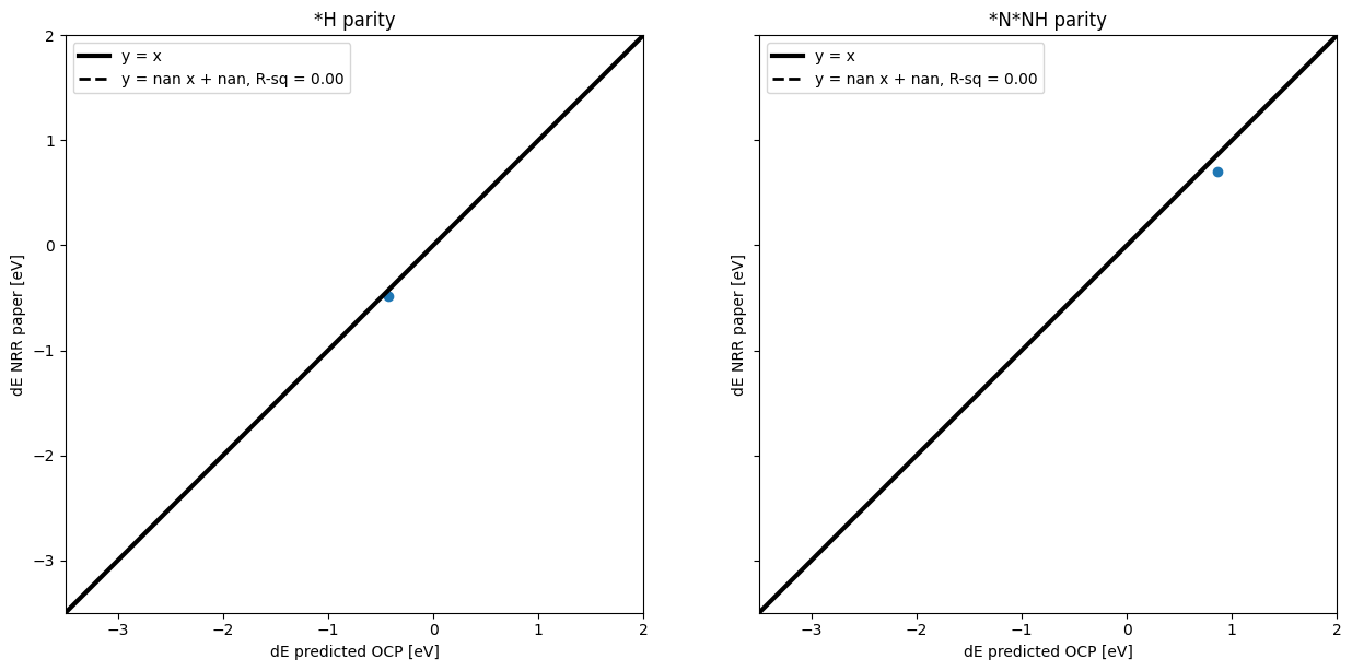
Make parity plots for values obtained by ML v. reported in the paper#
# Add literature data to the dataframe
with open("literature_data.pkl", "rb") as f:
    literature_data = pickle.load(f)
df_all = df_flat.merge(pd.DataFrame(literature_data), on = "bulk_id")
f, (ax1, ax2) = plt.subplots(1, 2, sharey=True)
f.set_figheight(15)
x = df_all.min_E_ml_x.tolist()
y = df_all.E_lit_H.tolist()
ax1.set_title("*H parity")
ax1.plot([-3.5, 2], [-3.5, 2], "k-", linewidth=3)
slope, intercept, r, p, se = linregress(x, y)
ax1.plot(
    [-3.5, 2],
    [
        -3.5 * slope + intercept,
        2 * slope + intercept,
    ],
    "k--",
    linewidth=2,
)

ax1.legend(
    [
        "y = x",
        f"y = {slope:1.2f} x + {intercept:1.2f}, R-sq = {r**2:1.2f}",
    ],
    loc="upper left",
)
ax1.scatter(x, y)
ax1.axis("square")
ax1.set_xlim([-3.5, 2])
ax1.set_ylim([-3.5, 2])
ax1.set_xlabel("dE predicted OCP [eV]")
ax1.set_ylabel("dE NRR paper [eV]");


x = df_all.min_E_ml_y.tolist()
y = df_all.E_lit_NNH.tolist()
ax2.set_title("*N*NH parity")
ax2.plot([-3.5, 2], [-3.5, 2], "k-", linewidth=3)
slope, intercept, r, p, se = linregress(x, y)
ax2.plot(
    [-3.5, 2],
    [
        -3.5 * slope + intercept,
        2 * slope + intercept,
    ],
    "k--",
    linewidth=2,
)

ax2.legend(
    [
        "y = x",
        f"y = {slope:1.2f} x + {intercept:1.2f}, R-sq = {r**2:1.2f}",
    ],
    loc="upper left",
)
ax2.scatter(x, y)
ax2.axis("square")
ax2.set_xlim([-3.5, 2])
ax2.set_ylim([-3.5, 2])
ax2.set_xlabel("dE predicted OCP [eV]")
ax2.set_ylabel("dE NRR paper [eV]");
f.set_figwidth(15)
f.set_figheight(7)
/opt/hostedtoolcache/Python/3.12.8/x64/lib/python3.12/site-packages/scipy/stats/_stats_py.py:10729: RuntimeWarning: invalid value encountered in scalar divide
  slope = ssxym / ssxm
/opt/hostedtoolcache/Python/3.12.8/x64/lib/python3.12/site-packages/scipy/stats/_stats_py.py:10743: RuntimeWarning: invalid value encountered in sqrt
  t = r * np.sqrt(df / ((1.0 - r + TINY)*(1.0 + r + TINY)))
/opt/hostedtoolcache/Python/3.12.8/x64/lib/python3.12/site-packages/scipy/stats/_stats_py.py:10749: RuntimeWarning: invalid value encountered in scalar divide
  slope_stderr = np.sqrt((1 - r**2) * ssym / ssxm / df)
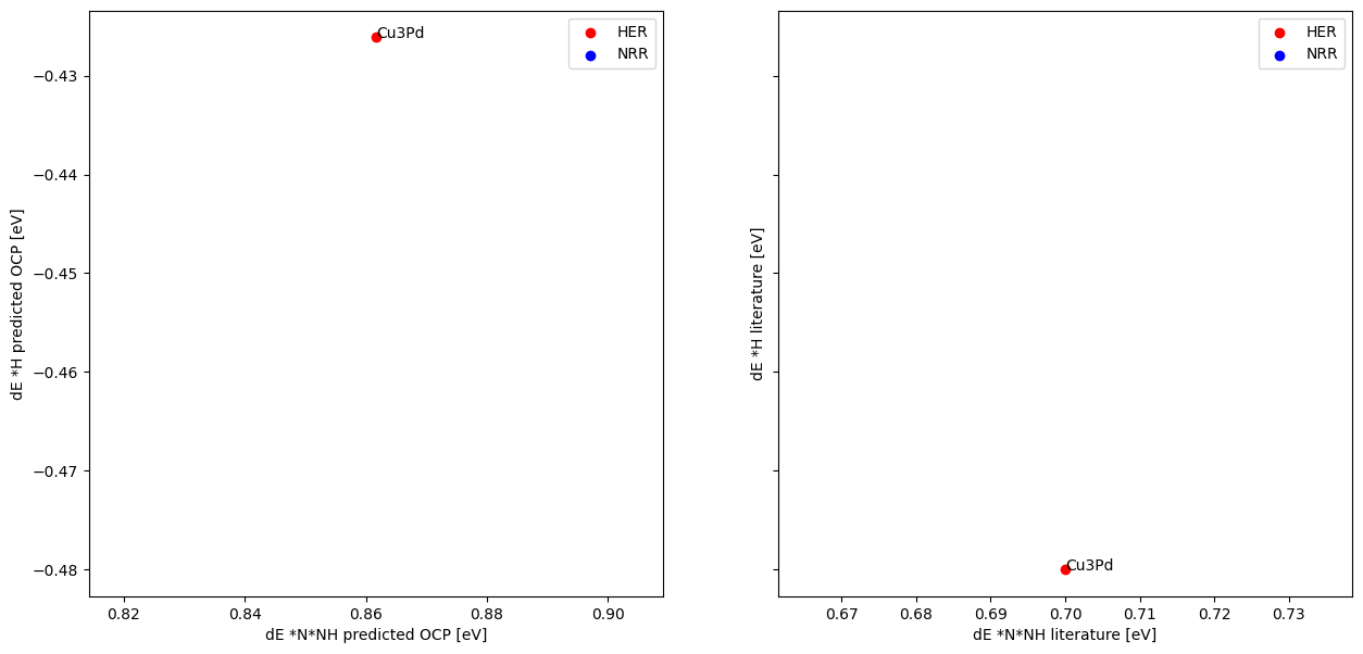
Make figure 6b and compare to literature results#
f, (ax1, ax2) = plt.subplots(1, 2, sharey=True)
x = df_all[df_all.reaction == "HER"].min_E_ml_y.tolist()
y = df_all[df_all.reaction == "HER"].min_E_ml_x.tolist()
comp = df_all[df_all.reaction == "HER"].composition.tolist()

ax1.scatter(x, y,c= "r", label = "HER")
for i, txt in enumerate(comp):
    ax1.annotate(txt, (x[i], y[i]))

x = df_all[df_all.reaction == "NRR"].min_E_ml_y.tolist()
y = df_all[df_all.reaction == "NRR"].min_E_ml_x.tolist()
comp = df_all[df_all.reaction == "NRR"].composition.tolist()
ax1.scatter(x, y,c= "b", label = "NRR")
for i, txt in enumerate(comp):
    ax1.annotate(txt, (x[i], y[i]))


ax1.legend()
ax1.set_xlabel("dE *N*NH predicted OCP [eV]")
ax1.set_ylabel("dE *H predicted OCP [eV]")


x = df_all[df_all.reaction == "HER"].E_lit_NNH.tolist()
y = df_all[df_all.reaction == "HER"].E_lit_H.tolist()
comp = df_all[df_all.reaction == "HER"].composition.tolist()

ax2.scatter(x, y,c= "r", label = "HER")
for i, txt in enumerate(comp):
    ax2.annotate(txt, (x[i], y[i]))

x = df_all[df_all.reaction == "NRR"].E_lit_NNH.tolist()
y = df_all[df_all.reaction == "NRR"].E_lit_H.tolist()
comp = df_all[df_all.reaction == "NRR"].composition.tolist()
ax2.scatter(x, y,c= "b", label = "NRR")
for i, txt in enumerate(comp):
    ax2.annotate(txt, (x[i], y[i]))

ax2.legend()
ax2.set_xlabel("dE *N*NH literature [eV]")
ax2.set_ylabel("dE *H literature [eV]")
f.set_figwidth(15)
f.set_figheight(7)