| Property | Value |
|---|---|
| Difficulty | Beginner |
| Time | 15-30 minutes |
| Prerequisites | Basic Python, familiarity with ASE |
| Goal | Calculate adsorption energies using UMA models |
To introduce OCP we start with using it to calculate adsorption energies for a simple, atomic adsorbate where we specify the site we want to the adsorption energy for. Conceptually, you do this like you would do it with density functional theory. You create a slab model for the surface, place an adsorbate on it as an initial guess, run a relaxation to get the lowest energy geometry, and then compute the adsorption energy using reference states for the adsorbate.
Intro to Adsorption energies
Adsorption energies are always a reaction energy (an adsorbed species relative to some implied combination of reactants). There are many common schemes in the catalysis literature.
For example, you may want the adsorption energy of oxygen, and you might compute that from this reaction:
1/2 O2 + slab -> slab-ODFT has known errors with the energy of a gas-phase O2 molecule, so it’s more common to compute this energy relative to a linear combination of H2O and H2. The suggested reference scheme for consistency with OC20 is a reaction
x CO + (x + y/2 - z) H2 + (z-x) H2O + w/2 N2 + * -> CxHyOzNw*Here, x=y=w=0, z=1, so the reaction ends up as
-H2 + H2O + * -> O*or alternatively,
H2O + * -> O* + H2It is possible through thermodynamic cycles to compute other reactions. If we can look up rH1 below and compute rH2
H2 + 1/2 O2 -> H2O  re1 = -3.03 eV, from exp
H2O + * -> O* + H2  re2  # Get from UMA
Then, the adsorption energy for
1/2O2 + * -> O*is just re1 + re2.
Based on https://atct.anl.gov/Thermochemical Data/version 1.118/species/?species_number=986, the formation energy of water is about -3.03 eV at standard state experimentally. You could also compute this using DFT, but you would probably get the wrong answer for this.
The first step is getting a checkpoint for the model we want to use. UMA is currently the state-of-the-art model and will provide total energy estimates at the RPBE level of theory if you use the “OC20” task.
Need to install fairchem-core or get UMA access or getting permissions/401 errors?
Install the necessary packages using pip, uv etc
! pip install fairchem-core fairchem-data-oc fairchem-applications-cattsunamiGet access to any necessary huggingface gated models
Get and login to your Huggingface account
Request access to https://
huggingface .co /facebook /UMA Create a Huggingface token at https://
huggingface .co /settings /tokens/ with the permission “Permissions: Read access to contents of all public gated repos you can access” Add the token as an environment variable using
huggingface-cli loginor by setting the HF_TOKEN environment variable.
# Login using the huggingface-cli utility
! huggingface-cli login

# alternatively,
import os
os.environ['HF_TOKEN'] = 'MY_TOKEN'
If you find your kernel is crashing, it probably means you have exceeded the allowed amount of memory. This checkpoint works fine in this example, but it may crash your kernel if you use it in the NRR example.
This next cell will automatically download the checkpoint from huggingface and load it.
from __future__ import annotations

from fairchem.core import FAIRChemCalculator, pretrained_mlip

predictor = pretrained_mlip.get_predict_unit("uma-s-1p2")
calc = FAIRChemCalculator(predictor, task_name="oc20")
WARNING:root:device was not explicitly set, using device='cuda'.
Next we can build a slab with an adsorbate on it. Here we use the ASE module to build a Pt slab. We use the experimental lattice constant that is the default. This can introduce some small errors with DFT since the lattice constant can differ by a few percent, and it is common to use DFT lattice constants. In this example, we do not constrain any layers.
from ase.build import add_adsorbate, fcc111
from ase.optimize import BFGS
# reference energies from a linear combination of H2O/N2/CO/H2!
atomic_reference_energies = {
"H": -3.477,
"N": -8.083,
"O": -7.204,
"C": -7.282,
}
re1 = -3.03
slab = fcc111("Pt", size=(2, 2, 5), vacuum=20.0)
slab.pbc = True
adslab = slab.copy()
add_adsorbate(adslab, "O", height=1.2, position="fcc")
slab.set_calculator(calc)
opt = BFGS(slab)
opt.run(fmax=0.05, steps=100)
slab_e = slab.get_potential_energy()
adslab.set_calculator(calc)
opt = BFGS(adslab)
opt.run(fmax=0.05, steps=100)
adslab_e = adslab.get_potential_energy()
# Energy for ((H2O-H2) + * -> *O) + (H2 + 1/2O2 -> H2) leads to 1/2O2 + * -> *O!
adslab_e - slab_e - atomic_reference_energies["O"] + re1/tmp/ipykernel_8521/3752951811.py:17: FutureWarning: Please use atoms.calc = calc
slab.set_calculator(calc)
      Step     Time          Energy          fmax
BFGS:    0 14:18:48     -104.694021        0.695050
BFGS:    1 14:18:48     -104.750471        0.597034
BFGS: 2 14:18:49 -104.896312 0.382719
BFGS: 3 14:18:49 -104.926056 0.441386
BFGS: 4 14:18:49 -105.022125 0.447649
BFGS: 5 14:18:49 -105.082321 0.322276
BFGS: 6 14:18:50 -105.111680 0.162513
BFGS: 7 14:18:50 -105.122293 0.038224
/tmp/ipykernel_8521/3752951811.py:22: FutureWarning: Please use atoms.calc = calc
  adslab.set_calculator(calc)
      Step     Time          Energy          fmax
BFGS:    0 14:18:50     -110.077201        1.746972
BFGS: 1 14:18:50 -110.258223 0.993460
BFGS: 2 14:18:51 -110.405518 0.740256
BFGS: 3 14:18:51 -110.453436 0.792026
BFGS: 4 14:18:51 -110.570003 0.602221
BFGS: 5 14:18:52 -110.638272 0.491857
BFGS: 6 14:18:52 -110.695130 0.598345
BFGS: 7 14:18:52 -110.741332 0.612750
BFGS: 8 14:18:53 -110.772909 0.428322
BFGS: 9 14:18:53 -110.788240 0.191989
BFGS: 10 14:18:53 -110.791606 0.095431
BFGS: 11 14:18:54 -110.792269 0.094852
BFGS: 12 14:18:54 -110.793024 0.085642
BFGS: 13 14:18:54 -110.793669 0.071266
BFGS: 14 14:18:55 -110.794200 0.053573
BFGS: 15 14:18:55 -110.794438 0.042701
-1.498145838553007It is good practice to look at your geometries to make sure they are what you expect.
import matplotlib.pyplot as plt
from ase.visualize.plot import plot_atoms

fig, axs = plt.subplots(1, 2)
plot_atoms(slab, axs[0])
plot_atoms(slab, axs[1], rotation=("-90x"))
axs[0].set_axis_off()
axs[1].set_axis_off()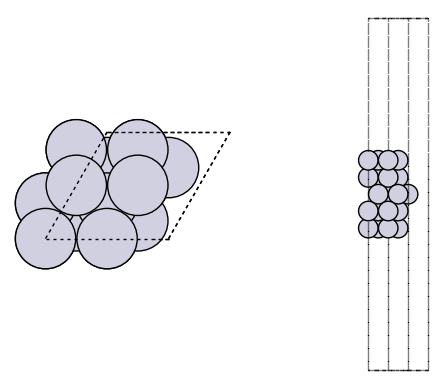
import matplotlib.pyplot as plt
from ase.visualize.plot import plot_atoms

fig, axs = plt.subplots(1, 2)
plot_atoms(adslab, axs[0])
plot_atoms(adslab, axs[1], rotation=("-90x"))
axs[0].set_axis_off()
axs[1].set_axis_off()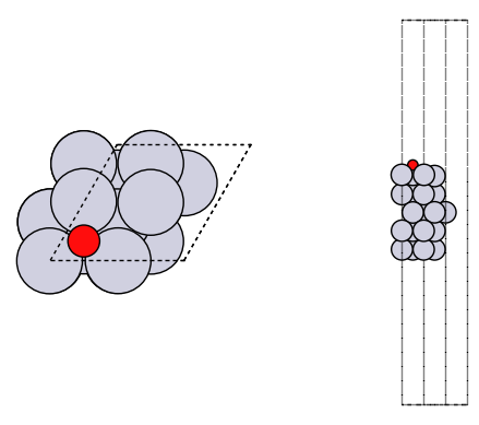
How did we do? We need a reference point. In the paper below, there is an atomic adsorption energy for O on Pt(111) of about -4.264 eV. This is for the reaction O + * -> O*. To convert this to the dissociative adsorption energy, we have to add the reaction:
1/2 O2 -> O D = 2.58 eV (expt)to get a comparable energy of about -1.68 eV. There is about ~0.2 eV difference (we predicted -1.47 eV above, and the reference comparison is -1.68 eV) to account for. The biggest difference is likely due to the differences in exchange-correlation functional. The reference data used the PBE functional, and eSCN was trained on RPBE data. To additional places where there are differences include:
Difference in lattice constant
The reference energy used for the experiment references. These can differ by up to 0.5 eV from comparable DFT calculations.
How many layers are relaxed in the calculation
Some of these differences tend to be systematic, and you can calibrate and correct these, especially if you can augment these with your own DFT calculations.
See convergence study for some additional studies of factors that influence this number.
Exercises
Explore the effect of the lattice constant on the adsorption energy.
Try different sites, including the bridge and top sites. Compare the energies, and inspect the resulting geometries.
Trends in adsorption energies across metals.
Xu, Z., & Kitchin, J. R. (2014). Probing the coverage dependence of site and adsorbate configurational correlations on (111) surfaces of late transition metals. J. Phys. Chem. C, 118(44), 25597–25602. Xu & Kitchin (2014)
These are atomic adsorption energies:
O + * -> O*We have to do some work to get comparable numbers from OCP
H2 + 1/2 O2 -> H2O  re1 = -3.03 eV
H2O + * -> O* + H2  re2   # Get from UMA
O -> 1/2 O2         re3 = -2.58 eV
Then, the adsorption energy for
O + * -> O*is just re1 + re2 + re3.
Here we just look at the fcc site on Pt. First, we get the data stored in the paper.
Next we get the structures and compute their energies. Some subtle points are that we have to account for stoichiometry, and normalize the adsorption energy by the number of oxygens.
First we get a reference energy from the paper (PBE, 0.25 ML O on Pt(111)).
import json

with open("energies.json") as f:
    edata = json.load(f)

with open("structures.json") as f:
    sdata = json.load(f)

edata["Pt"]["O"]["fcc"]["0.25"]-4.263842000000002Next, we load data from the SI to get the geometry to start from.
with open("structures.json") as f:
    s = json.load(f)

sfcc = s["Pt"]["O"]["fcc"]["0.25"]
Next, we construct the atomic geometry, run the geometry optimization, and compute the energy.
re3 = -2.58  # O -> 1/2 O2         re3 = -2.58 eV

from ase import Atoms

adslab = Atoms(sfcc["symbols"], positions=sfcc["pos"], cell=sfcc["cell"], pbc=True)

# Grab just the metal surface atoms
slab = adslab[adslab.arrays["numbers"] == adslab.arrays["numbers"][0]]
adsorbates = adslab[~(adslab.arrays["numbers"] == adslab.arrays["numbers"][0])]
slab.set_calculator(calc)
opt = BFGS(slab)
opt.run(fmax=0.05, steps=100)

adslab.set_calculator(calc)
opt = BFGS(adslab)

opt.run(fmax=0.05, steps=100)
re2 = (
    adslab.get_potential_energy()
    - slab.get_potential_energy()
    - sum([atomic_reference_energies[x] for x in adsorbates.get_chemical_symbols()])
)

nO = 0
for atom in adslab:
    if atom.symbol == "O":
        nO += 1
        re2 += re1 + re3

print(re2 / nO)
/tmp/ipykernel_8521/647904475.py:10: FutureWarning: Please use atoms.calc = calc
slab.set_calculator(calc)
      Step     Time          Energy          fmax
BFGS:    0 14:18:59      -82.881492        1.012517
BFGS: 1 14:18:59 -82.940117 0.758967
BFGS: 2 14:18:59 -83.035745 0.334363
BFGS:    3 14:18:59      -83.039932        0.304527
BFGS:    4 14:19:00      -83.049372        0.206965
BFGS: 5 14:19:00 -83.054435 0.140384
BFGS: 6 14:19:00 -83.057106 0.076570
BFGS: 7 14:19:00 -83.057955 0.064839
BFGS: 8 14:19:01 -83.058538 0.066527
BFGS: 9 14:19:01 -83.058831 0.045636
/tmp/ipykernel_8521/647904475.py:14: FutureWarning: Please use atoms.calc = calc
  adslab.set_calculator(calc)
      Step     Time          Energy          fmax
BFGS:    0 14:19:01      -88.773355        0.334878
BFGS: 1 14:19:01 -88.777414 0.290913
BFGS: 2 14:19:02 -88.789784 0.119410
BFGS: 3 14:19:02 -88.791837 0.124366
BFGS: 4 14:19:02 -88.795399 0.130637
BFGS: 5 14:19:03 -88.797986 0.118737
BFGS:    6 14:19:03      -88.800127        0.085204
BFGS:    7 14:19:03      -88.801290        0.091576
BFGS: 8 14:19:03 -88.802145 0.065006
BFGS: 9 14:19:04 -88.802709 0.042340
-4.149877723082704
Site correlations
This cell reproduces a portion of a figure in the paper. We compare oxygen adsorption energies in the fcc and hcp sites across metals and coverages. These adsorption energies are highly correlated with each other because the adsorption sites are so similar.
At higher coverages, the agreement is not as good. This is likely because the model is extrapolating and needs to be fine-tuned.
import time

from tqdm import tqdm

t0 = time.time()

data = {"fcc": [], "hcp": []}

refdata = {"fcc": [], "hcp": []}


for metal in ["Cu", "Ag", "Pd", "Pt", "Rh", "Ir"]:
    print(metal)
    for site in ["fcc", "hcp"]:
        for adsorbate in ["O"]:
            for coverage in tqdm(["0.25"]):

                entry = s[metal][adsorbate][site][coverage]

                adslab = Atoms(
                    entry["symbols"],
                    positions=entry["pos"],
                    cell=entry["cell"],
                    pbc=True,
                )

                # Grab just the metal surface atoms
                adsorbates = adslab[
                    ~(adslab.arrays["numbers"] == adslab.arrays["numbers"][0])
                ]

                slab = adslab[adslab.arrays["numbers"] == adslab.arrays["numbers"][0]]
                slab.set_calculator(calc)
                opt = BFGS(slab)
                opt.run(fmax=0.05, steps=100)

                adslab.set_calculator(calc)
                opt = BFGS(adslab)
                opt.run(fmax=0.05, steps=100)

                re2 = (
                    adslab.get_potential_energy()
                    - slab.get_potential_energy()
                    - sum(
                        [
                            atomic_reference_energies[x]
                            for x in adsorbates.get_chemical_symbols()
                        ]
                    )
                )

                nO = 0
                for atom in adslab:
                    if atom.symbol == "O":
                        nO += 1
                        re2 += re1 + re3

                data[site] += [re2 / nO]
                refdata[site] += [edata[metal][adsorbate][site][coverage]]

f"Elapsed time = {time.time() - t0} seconds"
Cu
0%| | 0/1 [00:00<?, ?it/s]/tmp/ipykernel_8521/1356342052.py:33: FutureWarning: Please use atoms.calc = calc
slab.set_calculator(calc)
      Step     Time          Energy          fmax
BFGS:    0 14:19:04      -48.890191        0.646801
BFGS:    1 14:19:04      -48.913215        0.542334
BFGS:    2 14:19:05      -48.978855        0.272943
BFGS:    3 14:19:05      -48.980963        0.248401
BFGS:    4 14:19:05      -48.989843        0.142195
BFGS: 5 14:19:05 -48.994133 0.109507
BFGS: 6 14:19:05 -48.995943 0.057373
BFGS: 7 14:19:06 -48.996412 0.052332
BFGS: 8 14:19:06 -48.996839 0.050481
BFGS: 9 14:19:06 -48.997190 0.037864
/tmp/ipykernel_8521/1356342052.py:37: FutureWarning: Please use atoms.calc = calc
  adslab.set_calculator(calc)
      Step     Time          Energy          fmax
BFGS:    0 14:19:06      -55.183791        0.317002
BFGS: 1 14:19:07 -55.186079 0.260545
BFGS:    2 14:19:07      -55.194759        0.163267
BFGS:    3 14:19:07      -55.196862        0.156293
BFGS: 4 14:19:07 -55.200265 0.089519
BFGS: 5 14:19:08 -55.202050 0.085342
BFGS:    6 14:19:08      -55.203481        0.085304
BFGS:    7 14:19:08      -55.204714        0.106559
BFGS:    8 14:19:08      -55.206074        0.098629
BFGS:    9 14:19:09      -55.206942        0.055605
100%|██████████| 1/1 [00:04<00:00, 4.95s/it]100%|██████████| 1/1 [00:04<00:00, 4.95s/it]
BFGS: 10 14:19:09 -55.207302 0.041437
0%| | 0/1 [00:00<?, ?it/s] Step Time Energy fmax
BFGS: 0 14:19:09 -48.915497 0.555938
BFGS: 1 14:19:09 -48.933106 0.473539
BFGS: 2 14:19:09 -48.987176 0.208265
BFGS: 3 14:19:10 -48.988350 0.196053
BFGS:    4 14:19:10      -48.996556        0.040858
      Step     Time          Energy          fmax
BFGS:    0 14:19:10      -55.087818        0.314616
BFGS: 1 14:19:10 -55.089884 0.253627
BFGS:    2 14:19:10      -55.096718        0.155816
BFGS:    3 14:19:11      -55.098611        0.158030
BFGS: 4 14:19:11 -55.101906 0.102147
BFGS:    5 14:19:11      -55.103300        0.061644
BFGS:    6 14:19:11      -55.104082        0.058925
BFGS:    7 14:19:11      -55.104754        0.080595
BFGS:    8 14:19:11      -55.105736        0.089875
BFGS:    9 14:19:11      -55.106588        0.063167
100%|██████████| 1/1 [00:02<00:00, 2.78s/it]100%|██████████| 1/1 [00:02<00:00, 2.78s/it]
BFGS:   10 14:19:11      -55.106975        0.033877
Ag
0%| | 0/1 [00:00<?, ?it/s] Step Time Energy fmax
BFGS: 0 14:19:12 -33.015774 0.626056
BFGS: 1 14:19:12 -33.034755 0.545928
BFGS:    2 14:19:12      -33.103217        0.188722
BFGS:    3 14:19:12      -33.104919        0.179778
BFGS:    4 14:19:12      -33.106624        0.166504
BFGS:    5 14:19:13      -33.109909        0.127307
BFGS:    6 14:19:13      -33.113531        0.109333
BFGS:    7 14:19:13      -33.115653        0.053176
BFGS:    8 14:19:13      -33.116104        0.039456
      Step     Time          Energy          fmax
BFGS:    0 14:19:13      -38.158732        0.127417
BFGS:    1 14:19:13      -38.159782        0.119851
BFGS:    2 14:19:13      -38.170046        0.074139
BFGS:    3 14:19:14      -38.171023        0.083948
BFGS:    4 14:19:14      -38.174080        0.098325
BFGS:    5 14:19:14      -38.176470        0.091280
BFGS:    6 14:19:14      -38.178596        0.074026
BFGS:    7 14:19:14      -38.179924        0.083171
BFGS:    8 14:19:15      -38.180629        0.065162
BFGS:    9 14:19:15      -38.180974        0.037548
100%|██████████| 1/1 [00:03<00:00, 3.22s/it]100%|██████████| 1/1 [00:03<00:00, 3.22s/it]
0%| | 0/1 [00:00<?, ?it/s] Step Time Energy fmax
BFGS: 0 14:19:15 -33.037808 0.552148
BFGS: 1 14:19:15 -33.052341 0.486542
BFGS:    2 14:19:15      -33.108824        0.155455
BFGS:    3 14:19:16      -33.109719        0.145457
BFGS: 4 14:19:16 -33.111363 0.118068
BFGS: 5 14:19:16 -33.113395 0.079859
BFGS: 6 14:19:16 -33.115417 0.053419
BFGS:    7 14:19:16      -33.116024        0.030041
      Step     Time          Energy          fmax
BFGS:    0 14:19:17      -38.073489        0.119079
BFGS: 1 14:19:17 -38.074444 0.115486
BFGS: 2 14:19:17 -38.085486 0.074974
BFGS:    3 14:19:17      -38.086455        0.080958
BFGS:    4 14:19:17      -38.088452        0.081859
BFGS: 5 14:19:18 -38.089967 0.070828
100%|██████████| 1/1 [00:03<00:00, 3.28s/it]100%|██████████| 1/1 [00:03<00:00, 3.28s/it]
BFGS:    6 14:19:18      -38.091906        0.042959
Pd
0%| | 0/1 [00:00<?, ?it/s] Step Time Energy fmax
BFGS: 0 14:19:18 -70.174811 0.646926
BFGS: 1 14:19:18 -70.200771 0.520373
BFGS:    2 14:19:18      -70.253580        0.195411
BFGS:    3 14:19:19      -70.255195        0.188046
BFGS:    4 14:19:19      -70.262549        0.137567
BFGS:    5 14:19:19      -70.265012        0.106892
BFGS:    6 14:19:19      -70.266656        0.074818
BFGS:    7 14:19:19      -70.267604        0.061564
BFGS:    8 14:19:19      -70.268390        0.035466
      Step     Time          Energy          fmax
BFGS:    0 14:19:19      -76.139648        0.221609
BFGS: 1 14:19:19 -76.142815 0.197612
BFGS: 2 14:19:20 -76.157140 0.181487
BFGS: 3 14:19:20 -76.159369 0.159805
BFGS: 4 14:19:20 -76.163719 0.132237
BFGS: 5 14:19:20 -76.166339 0.105134
BFGS: 6 14:19:21 -76.168581 0.099639
BFGS: 7 14:19:21 -76.169880 0.098481
BFGS:    8 14:19:21      -76.170694        0.077169
BFGS:    9 14:19:21      -76.171128        0.049108
100%|██████████| 1/1 [00:03<00:00, 3.18s/it]100%|██████████| 1/1 [00:03<00:00, 3.18s/it]
0%| | 0/1 [00:00<?, ?it/s] Step Time Energy fmax
BFGS: 0 14:19:21 -70.208058 0.465459
BFGS: 1 14:19:21 -70.222887 0.381518
BFGS:    2 14:19:22      -70.257807        0.181341
BFGS:    3 14:19:22      -70.259016        0.170180
BFGS:    4 14:19:22      -70.266016        0.073012
BFGS:    5 14:19:22      -70.266661        0.070115
BFGS:    6 14:19:22      -70.267867        0.048795
      Step     Time          Energy          fmax
BFGS:    0 14:19:22      -75.957684        0.183791
BFGS:    1 14:19:22      -75.960869        0.164287
BFGS:    2 14:19:23      -75.970372        0.169075
BFGS:    3 14:19:23      -75.972327        0.164642
BFGS: 4 14:19:23 -75.977418 0.120430
BFGS: 5 14:19:23 -75.979833 0.110607
BFGS:    6 14:19:23      -75.981659        0.082724
BFGS:    7 14:19:24      -75.982830        0.078025
100%|██████████| 1/1 [00:02<00:00, 2.63s/it]100%|██████████| 1/1 [00:02<00:00, 2.63s/it]
BFGS:    8 14:19:24      -75.983553        0.046148
Pt
0%| | 0/1 [00:00<?, ?it/s] Step Time Energy fmax
BFGS: 0 14:19:24 -82.881492 1.012517
BFGS: 1 14:19:24 -82.940117 0.758968
BFGS:    2 14:19:24      -83.035745        0.334363
BFGS:    3 14:19:24      -83.039931        0.304531
BFGS:    4 14:19:25      -83.049371        0.206967
BFGS:    5 14:19:25      -83.054436        0.140387
BFGS: 6 14:19:25 -83.057105 0.076584
BFGS: 7 14:19:25 -83.057955 0.064845
BFGS: 8 14:19:25 -83.058537 0.066520
BFGS: 9 14:19:26 -83.058829 0.045640
      Step     Time          Energy          fmax
BFGS:    0 14:19:26      -88.773355        0.334878
BFGS:    1 14:19:26      -88.777413        0.290913
BFGS: 2 14:19:26 -88.789784 0.119410
BFGS: 3 14:19:27 -88.791839 0.124354
BFGS: 4 14:19:27 -88.795398 0.130637
BFGS: 5 14:19:27 -88.797986 0.118738
BFGS: 6 14:19:27 -88.800128 0.085211
BFGS: 7 14:19:28 -88.801290 0.091580
BFGS:    8 14:19:28      -88.802145        0.064995
BFGS:    9 14:19:28      -88.802709        0.042339
100%|██████████| 1/1 [00:04<00:00, 4.23s/it]100%|██████████| 1/1 [00:04<00:00, 4.24s/it]
0%| | 0/1 [00:00<?, ?it/s] Step Time Energy fmax
BFGS: 0 14:19:28 -82.968454 0.688065
BFGS: 1 14:19:28 -82.995521 0.558978
BFGS:    2 14:19:29      -83.049826        0.200180
BFGS:    3 14:19:29      -83.051294        0.185780
BFGS: 4 14:19:29 -83.057463 0.066861
BFGS:    5 14:19:29      -83.057909        0.055436
BFGS:    6 14:19:29      -83.058685        0.031715
      Step     Time          Energy          fmax
BFGS:    0 14:19:30      -88.396681        0.203984
BFGS:    1 14:19:30      -88.400062        0.174390
BFGS:    2 14:19:30      -88.408719        0.136409
BFGS:    3 14:19:30      -88.410332        0.134069
BFGS:    4 14:19:30      -88.414336        0.095111
BFGS:    5 14:19:30      -88.415783        0.090168
BFGS:    6 14:19:31      -88.417002        0.104753
BFGS:    7 14:19:31      -88.417817        0.094186
BFGS: 8 14:19:31 -88.418372 0.051463
100%|██████████| 1/1 [00:03<00:00, 3.23s/it]100%|██████████| 1/1 [00:03<00:00, 3.23s/it]
BFGS:    9 14:19:31      -88.418639        0.031992
Rh
0%| | 0/1 [00:00<?, ?it/s] Step Time Energy fmax
BFGS: 0 14:19:32 -100.191090 0.703650
BFGS: 1 14:19:32 -100.219546 0.608665
BFGS:    2 14:19:32     -100.286016        0.178447
BFGS:    3 14:19:32     -100.289172        0.138492
BFGS:    4 14:19:32     -100.299063        0.074326
BFGS:    5 14:19:32     -100.300011        0.067007
BFGS:    6 14:19:32     -100.301061        0.062659
BFGS:    7 14:19:33     -100.301787        0.049569
      Step     Time          Energy          fmax
BFGS:    0 14:19:33     -106.949006        0.238786
BFGS:    1 14:19:33     -106.954055        0.199552
BFGS:    2 14:19:33     -106.963647        0.066008
BFGS:    3 14:19:33     -106.963942        0.058097
100%|██████████| 1/1 [00:01<00:00, 1.94s/it]100%|██████████| 1/1 [00:01<00:00, 1.94s/it]
BFGS: 4 14:19:33 -106.964804 0.029321
0%| | 0/1 [00:00<?, ?it/s] Step Time Energy fmax
BFGS: 0 14:19:33 -100.169507 0.774354
BFGS: 1 14:19:34 -100.204661 0.634293
BFGS:    2 14:19:34     -100.287442        0.228392
BFGS:    3 14:19:34     -100.290399        0.177253
BFGS:    4 14:19:34     -100.298468        0.080626
BFGS:    5 14:19:34     -100.299793        0.067135
BFGS:    6 14:19:34     -100.300911        0.052083
BFGS:    7 14:19:35     -100.301598        0.051978
BFGS:    8 14:19:35     -100.302239        0.043626
      Step     Time          Energy          fmax
BFGS:    0 14:19:35     -106.904528        0.271607
BFGS:    1 14:19:35     -106.909937        0.214886
BFGS:    2 14:19:35     -106.920133        0.083912
BFGS:    3 14:19:35     -106.920387        0.076302
100%|██████████| 1/1 [00:02<00:00, 2.20s/it]100%|██████████| 1/1 [00:02<00:00, 2.20s/it]
BFGS:    4 14:19:35     -106.921196        0.030128
Ir
0%| | 0/1 [00:00<?, ?it/s] Step Time Energy fmax
BFGS: 0 14:19:36 -124.226220 1.208047
BFGS: 1 14:19:36 -124.303068 0.944243
BFGS: 2 14:19:36 -124.413829 0.177421
BFGS: 3 14:19:36 -124.417069 0.150391
BFGS: 4 14:19:36 -124.423699 0.053159
BFGS: 5 14:19:36 -124.424242 0.050764
BFGS: 6 14:19:37 -124.424756 0.044990
      Step     Time          Energy          fmax
BFGS:    0 14:19:37     -130.642842        0.410127
BFGS: 1 14:19:37 -130.656118 0.294537
BFGS: 2 14:19:37 -130.672540 0.084505
BFGS:    3 14:19:37     -130.673412        0.070182
BFGS:    4 14:19:38     -130.674100        0.062828
BFGS:    5 14:19:38     -130.675014        0.055398
BFGS:    6 14:19:38     -130.675473        0.050562
100%|██████████| 1/1 [00:02<00:00, 2.70s/it]100%|██████████| 1/1 [00:02<00:00, 2.70s/it]
BFGS: 7 14:19:38 -130.675726 0.043155
0%| | 0/1 [00:00<?, ?it/s] Step Time Energy fmax
BFGS: 0 14:19:38 -124.219231 1.178119
BFGS: 1 14:19:39 -124.302855 0.920684
BFGS: 2 14:19:39 -124.415676 0.214575
BFGS: 3 14:19:39 -124.418175 0.200550
BFGS:    4 14:19:39     -124.424014        0.075790
BFGS:    5 14:19:39     -124.424557        0.045441
      Step     Time          Energy          fmax
BFGS:    0 14:19:40     -130.530228        0.471262
BFGS:    1 14:19:40     -130.546421        0.333597
BFGS: 2 14:19:40 -130.565047 0.073568
BFGS: 3 14:19:40 -130.566054 0.078632
BFGS: 4 14:19:40 -130.566520 0.069134
BFGS: 5 14:19:41 -130.567330 0.073885
BFGS: 6 14:19:41 -130.567673 0.065454
100%|██████████| 1/1 [00:03<00:00, 3.10s/it]100%|██████████| 1/1 [00:03<00:00, 3.10s/it]BFGS: 7 14:19:41 -130.567875 0.043097
'Elapsed time = 37.50602865219116 seconds'First, we compare the computed data and reference data. There is a systematic difference of about 0.5 eV due to the difference between RPBE and PBE functionals, and other subtle differences like lattice constant differences and reference energy differences. This is pretty typical, and an expected deviation.
plt.plot(refdata["fcc"], data["fcc"], "r.", label="fcc")
plt.plot(refdata["hcp"], data["hcp"], "b.", label="hcp")
plt.plot([-5.5, -3.5], [-5.5, -3.5], "k-")
plt.xlabel("Ref. data (DFT)")
plt.ylabel("UMA-OC20 prediction");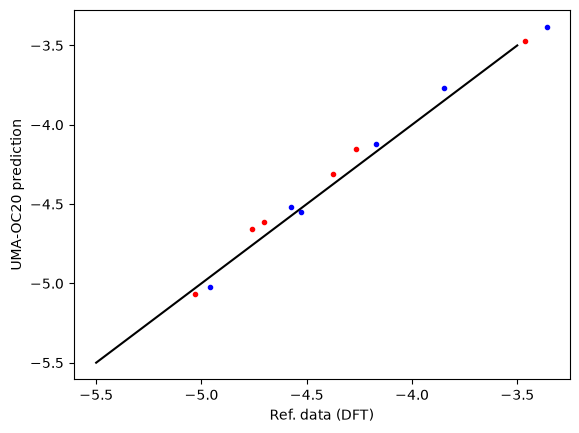
Next we compare the correlation between the hcp and fcc sites. Here we see the same trends. The data falls below the parity line because the hcp sites tend to be a little weaker binding than the fcc sites.
plt.plot(refdata["hcp"], refdata["fcc"], "r.")
plt.plot(data["hcp"], data["fcc"], ".")
plt.plot([-6, -1], [-6, -1], "k-")
plt.xlabel("$H_{ads, hcp}$")
plt.ylabel("$H_{ads, fcc}$")
plt.legend(["DFT (PBE)", "UMA-OC20"]);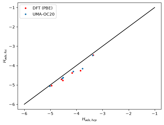
Exercises
You can also explore a few other adsorbates: C, H, N.
Explore the higher coverages. The deviations from the reference data are expected to be higher, but relative differences tend to be better. You probably need fine tuning to improve this performance. This data set doesn’t have forces though, so it isn’t practical to do it here.
Next steps
In the next step, we consider some more complex adsorbates in nitrogen reduction, and how we can leverage OCP to automate the search for the most stable adsorbate geometry. See the next step.
Convergence study
In the adsorption energies section we discussed some possible reasons we might see a discrepancy. Here we investigate some factors that impact the computed energies.
In this section, the energies refer to the reaction 1/2 O2 -> O*.
Effects of number of layers
Slab thickness could be a factor. Here we relax the whole slab, and see by about 4 layers the energy is converged to ~0.02 eV.
for nlayers in [3, 4, 5, 6, 7, 8]:
    slab = fcc111("Pt", size=(2, 2, nlayers), vacuum=10.0)

    slab.pbc = True
    slab.set_calculator(calc)
    opt_slab = BFGS(slab, logfile=None)
    opt_slab.run(fmax=0.05, steps=100)
    slab_e = slab.get_potential_energy()

    adslab = slab.copy()
    add_adsorbate(adslab, "O", height=1.2, position="fcc")

    adslab.pbc = True
    adslab.set_calculator(calc)
    opt_adslab = BFGS(adslab, logfile=None)
    opt_adslab.run(fmax=0.05, steps=100)
    adslab_e = adslab.get_potential_energy()

    print(
        f"nlayers = {nlayers}: {adslab_e - slab_e - atomic_reference_energies['O'] + re1:1.2f} eV"
    )
/tmp/ipykernel_8521/338101817.py:5: FutureWarning: Please use atoms.calc = calc
slab.set_calculator(calc)
/tmp/ipykernel_8521/338101817.py:14: FutureWarning: Please use atoms.calc = calc
  adslab.set_calculator(calc)
nlayers = 3: -1.64 eV
nlayers = 4: -1.47 eV
nlayers = 5: -1.50 eV
nlayers = 6: -1.48 eV
nlayers = 7: -1.49 eV
nlayers = 8: -1.49 eV
Effects of relaxation
It is common to only relax a few layers, and constrain lower layers to bulk coordinates. We do that here. We only relax the adsorbate and the top layer.
This has a small effect (0.1 eV).
from ase.constraints import FixAtoms

for nlayers in [3, 4, 5, 6, 7, 8]:
    slab = fcc111("Pt", size=(2, 2, nlayers), vacuum=10.0)

    slab.set_constraint(FixAtoms(mask=[atom.tag > 1 for atom in slab]))
    slab.pbc = True
    slab.set_calculator(calc)
    opt_slab = BFGS(slab, logfile=None)
    opt_slab.run(fmax=0.05, steps=100)
    slab_e = slab.get_potential_energy()

    adslab = slab.copy()
    add_adsorbate(adslab, "O", height=1.2, position="fcc")

    adslab.set_constraint(FixAtoms(mask=[atom.tag > 1 for atom in adslab]))
    adslab.pbc = True
    adslab.set_calculator(calc)
    opt_adslab = BFGS(adslab, logfile=None)
    opt_adslab.run(fmax=0.05, steps=100)
    adslab_e = adslab.get_potential_energy()

    print(
        f"nlayers = {nlayers}: {adslab_e - slab_e - atomic_reference_energies['O'] + re1:1.2f} eV"
    )
/tmp/ipykernel_8521/1426773950.py:8: FutureWarning: Please use atoms.calc = calc
slab.set_calculator(calc)
/tmp/ipykernel_8521/1426773950.py:18: FutureWarning: Please use atoms.calc = calc
  adslab.set_calculator(calc)
nlayers = 3: -1.54 eV
nlayers = 4: -1.35 eV
nlayers = 5: -1.38 eV
nlayers = 6: -1.37 eV
nlayers = 7: -1.38 eV
nlayers = 8: -1.38 eV
Unit cell size
Coverage effects are quite noticeable with oxygen. Here we consider larger unit cells. This effect is large, and the results don’t look right, usually adsorption energies get more favorable at lower coverage, not less. This suggests fine-tuning could be important even at low coverages.
for size in [1, 2, 3, 4, 5]:

    slab = fcc111("Pt", size=(size, size, 5), vacuum=10.0)

    slab.set_constraint(FixAtoms(mask=[atom.tag > 1 for atom in slab]))
    slab.pbc = True
    slab.set_calculator(calc)
    opt_slab = BFGS(slab, logfile=None)
    opt_slab.run(fmax=0.05, steps=100)
    slab_e = slab.get_potential_energy()

    adslab = slab.copy()
    add_adsorbate(adslab, "O", height=1.2, position="fcc")

    adslab.set_constraint(FixAtoms(mask=[atom.tag > 1 for atom in adslab]))
    adslab.pbc = True
    adslab.set_calculator(calc)
    opt_adslab = BFGS(adslab, logfile=None)
    opt_adslab.run(fmax=0.05, steps=100)
    adslab_e = adslab.get_potential_energy()

    print(
        f"({size}x{size}): {adslab_e - slab_e - atomic_reference_energies['O'] + re1:1.2f} eV"
    )
/tmp/ipykernel_8521/3371624330.py:7: FutureWarning: Please use atoms.calc = calc
slab.set_calculator(calc)
/tmp/ipykernel_8521/3371624330.py:17: FutureWarning: Please use atoms.calc = calc
  adslab.set_calculator(calc)
(1x1): -0.22 eV
(2x2): -1.38 eV
(3x3): -1.43 eV
(4x4): -1.45 eV
(5x5): -1.46 eV
Summary
As with DFT, you should take care to see how these kinds of decisions affect your results, and determine if they would change any interpretations or not.
- Xu, Z., & Kitchin, J. R. (2014). Probing the Coverage Dependence of Site and Adsorbate Configurational Correlations on (111) Surfaces of Late Transition Metals. The Journal of Physical Chemistry C, 118(44), 25597–25602. 10.1021/jp508805h