UMA Intro Tutorial - FAIR Chemistry Documentation

This tutorial will walk you through a few examples of how you can use UMA. Each step is covered in more detail elsewhere in the documentation, but this is well suited to a ~1-2 hour tutorial session for researchers new to UMA but with some background in ASE and molecular simulations.

Before you start / installation¶

You need to get a HuggingFace account and request access to the UMA models.

You need a Huggingface account, request access to https://huggingface.co/facebook/UMA, and to create a Huggingface token at https://huggingface.co/settings/tokens/ with these permission:

Permissions: Read access to contents of all public gated repos you can access

Then, add the token as an environment variable (using huggingface-cli login:

# Enter token via huggingface-cli
! huggingface-cli login

or you can set the token via HF_TOKEN variable:

# Set token via env variable
import os
os.environ['HF_TOKEN'] = 'MYTOKEN'

Installation process¶

It may be enough to use pip install fairchem-core. This gets you the latest version on PyPi (https://pypi.org/project/fairchem-core/)

Here we install some sub-packages. This can take 2-5 minutes to run.

! pip install fairchem-core fairchem-data-oc fairchem-applications-cattsunami x3dase

# Check that packages are installed
!pip list | grep fairchem

fairchem-applications-cattsunami   1.1.2.dev239+g171971183
fairchem-core                      2.18.0
fairchem-data-oc                   1.0.3.dev239+g171971183
fairchem-data-omat                 0.2.1.dev144+g171971183

import fairchem.core

fairchem.core.__version__

Warp DeprecationWarning: The symbol `warp.vec` will soon be removed from the public API. Use `warp.types.vector` instead.

'2.18.0'

Illustrative examples¶

These should just run, and are here to show some basic uses.

Spin gap energy - OMOL¶

This is the difference in energy between a triplet and single ground state for a CH2 radical. This downloads a ~1GB checkpoint the first time you run it.

OMOL Task Requirements

For molecular calculations with the omol task, you must set spin and charge in atoms.info:

atoms.info.update({"spin": 1, "charge": 0})

Spin is the multiplicity (1 for singlet, 2 for doublet, 3 for triplet, etc.).

We don’t set a device here, so we get a warning about using a CPU device. You can ignore that. If a CUDA environment is available, a GPU may be used to speed up the calculations.

from fairchem.core import FAIRChemCalculator, pretrained_mlip

predictor = pretrained_mlip.get_predict_unit("uma-s-1")

---------------------------------------------------------------------------
KeyError                                  Traceback (most recent call last)
File ~/work/_tool/Python/3.12.13/x64/lib/python3.12/site-packages/fairchem/core/calculate/pretrained_mlip.py:54, in pretrained_checkpoint_path_from_name(model_name)
     53 try:
---> 54     model_checkpoint = _MODEL_CKPTS.checkpoints[model_name]
     55 except KeyError as err:

KeyError: 'uma-s-1'

The above exception was the direct cause of the following exception:

KeyError                                  Traceback (most recent call last)
Cell In[3], line 3
      1 from fairchem.core import FAIRChemCalculator, pretrained_mlip
----> 3 predictor = pretrained_mlip.get_predict_unit("uma-s-1")

File ~/work/_tool/Python/3.12.13/x64/lib/python3.12/site-packages/fairchem/core/calculate/pretrained_mlip.py:97, in get_predict_unit(model_name, inference_settings, overrides, device, cache_dir, workers)
     69 def get_predict_unit(
     70     model_name: str,
     71     inference_settings: InferenceSettings | str = "default",
   (...)     75     workers: int = 1,
     76 ) -> MLIPPredictUnit:
     77     """
     78     Retrieves a prediction unit for a specified model.
     79 
   (...)     95         KeyError: If the specified model_name is not found in available models.
     96     """
---> 97     checkpoint_path = pretrained_checkpoint_path_from_name(model_name)
     98     atom_refs = get_reference_energies(model_name, "atom_refs", cache_dir)
    100     if _MODEL_CKPTS.checkpoints[model_name].form_elem_refs is not None:

File ~/work/_tool/Python/3.12.13/x64/lib/python3.12/site-packages/fairchem/core/calculate/pretrained_mlip.py:56, in pretrained_checkpoint_path_from_name(model_name)
     54     model_checkpoint = _MODEL_CKPTS.checkpoints[model_name]
     55 except KeyError as err:
---> 56     raise KeyError(
     57         f"Model '{model_name}' not found. Available models: {available_models}"
     58     ) from err
     59 checkpoint_path = hf_hub_download(
     60     filename=model_checkpoint.filename,
     61     repo_id=model_checkpoint.repo_id,
   (...)     64     cache_dir=CACHE_DIR,
     65 )
     66 return checkpoint_path

KeyError: "Model 'uma-s-1' not found. Available models: ('uma-s-1p2', 'uma-s-1p1', 'uma-m-1p1', 'esen-md-direct-all-omol', 'esen-sm-conserving-all-omol', 'esen-sm-direct-all-omol', 'esen-sm-conserving-all-oc25', 'esen-md-direct-all-oc25', 'esen-sm-filtered-odac25', 'esen-sm-full-odac25')"

from ase.build import molecule

#  singlet CH2
singlet = molecule("CH2_s1A1d")
singlet.info.update({"spin": 1, "charge": 0})
singlet.calc = FAIRChemCalculator(predictor, task_name="omol")

#  triplet CH2
triplet = molecule("CH2_s3B1d")
triplet.info.update({"spin": 3, "charge": 0})
triplet.calc = FAIRChemCalculator(predictor, task_name="omol")

print(triplet.get_potential_energy() - singlet.get_potential_energy())

Example of adsorbate relaxation - OC20¶

Here we just setup a Cu(100) slab with a CO on it and relax it.

We specify an explicit device in the predictor here, and avoid the warning.

from ase.build import add_adsorbate, fcc100, molecule
from ase.optimize import LBFGS
from fairchem.core import FAIRChemCalculator, pretrained_mlip

predictor = pretrained_mlip.get_predict_unit("uma-s-1")
calc = FAIRChemCalculator(predictor, task_name="oc20")

# Set up your system as an ASE atoms object
slab = fcc100("Cu", (3, 3, 3), vacuum=8, periodic=True)

adsorbate = molecule("CO")
add_adsorbate(slab, adsorbate, 2.0, "bridge")
slab.calc = calc

# Set up LBFGS dynamics object
opt = LBFGS(slab)
opt.run(0.05, 100)
print(slab.get_potential_energy())

Example bulk relaxation - OMAT¶

from ase.build import bulk
from ase.filters import FrechetCellFilter
from ase.optimize import FIRE
from fairchem.core import FAIRChemCalculator, pretrained_mlip

predictor = pretrained_mlip.get_predict_unit("uma-s-1")
calc = FAIRChemCalculator(predictor, task_name="omat")

atoms = bulk("Fe")
atoms.calc = calc

opt = FIRE(FrechetCellFilter(atoms))
opt.run(0.05, 100)

print(atoms.get_stress())  # !!!! We get stress now!

Molecular dynamics - OMOL¶

import matplotlib.pyplot as plt

from ase import units
from ase.build import molecule
from ase.io import Trajectory
from ase.md.langevin import Langevin
from fairchem.core import FAIRChemCalculator, pretrained_mlip

predictor = pretrained_mlip.get_predict_unit("uma-s-1")
calc = FAIRChemCalculator(predictor, task_name="omol")

atoms = molecule("H2O")
atoms.info.update(charge=0, spin=1)  # For omol

atoms.calc = calc

dyn = Langevin(
    atoms,
    timestep=0.1 * units.fs,
    temperature_K=400,
    friction=0.001 / units.fs,
)

trajectory = Trajectory("my_md.traj", "w", atoms)
dyn.attach(trajectory.write, interval=1)
dyn.run(steps=50)

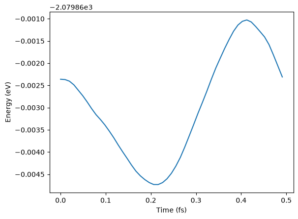
# See some results - not paper ready!
traj = Trajectory("my_md.traj")
plt.plot(
    [i * 0.1 * units.fs for i in range(len(traj))],
    [a.get_potential_energy() for a in traj],
)
plt.xlabel("Time (fs)")
plt.ylabel("Energy (eV)");

Catalyst Adsorption energies¶

The basic approach in computing an adsorption energy is to compute this energy difference:

dH = E_adslab - E_slab - E_ads

We use UMA for two of these energies E_adslab and E_slab. For E_ads We have to do something a little different. The OC20 task is not trained for molecules or molecular fragments. We use atomic energy reference energies instead. These are tabulated below.

The OC20 reference scheme is this reaction:

x CO + (x + y/2 - z) H2 + (z-x) H2O + w/2 N2 + * -> CxHyOzNw*

For this example we have

-H2 + H2O + * -> O*.   "O": -7.204 eV

Where "O": -7.204 is a constant.

To get the desired reaction energy we want we add the formation energy of water. We use either DFT or experimental values for this reaction energy.

1/2O2 + H2 -> H2O

Alternatives to this approach are using DFT to estimate the energy of 1/2 O2, just make sure to use consistent settings with your task. You should not use OMOL for this.

from ase.build import add_adsorbate, fcc111
from ase.optimize import BFGS
from fairchem.core import FAIRChemCalculator, pretrained_mlip

predictor = pretrained_mlip.get_predict_unit("uma-s-1")
calc = FAIRChemCalculator(predictor, task_name="oc20")

# reference energies from a linear combination of H2O/N2/CO/H2!
atomic_reference_energies = {
    "H": -3.477,
    "N": -8.083,
    "O": -7.204,
    "C": -7.282,
}

re1 = -3.03  # Water formation energy from experiment

slab = fcc111("Pt", size=(2, 2, 5), vacuum=20.0)
slab.pbc = True

adslab = slab.copy()
add_adsorbate(adslab, "O", height=1.2, position="fcc")

slab.calc = calc
opt = BFGS(slab)
print("Relaxing slab")
opt.run(fmax=0.05, steps=100)
slab_e = slab.get_potential_energy()

adslab.calc = calc
opt = BFGS(adslab)
print("\nRelaxing adslab")
opt.run(fmax=0.05, steps=100)
adslab_e = adslab.get_potential_energy()

Now we compute the adsorption energy.

# Energy for ((H2O-H2) + * -> *O) + (H2 + 1/2O2 -> H2O) leads to 1/2O2 + * -> *O!
adslab_e - slab_e - atomic_reference_energies["O"] + re1

How did we do? We need a reference point. In the paper below, there is an atomic adsorption energy for O on Pt(111) of about -4.264 eV. This is for the reaction O + * -> O*. To convert this to the dissociative adsorption energy, we have to add the reaction:

1/2 O2 -> O   D = 2.58 eV (expt)

to get a comparable energy of about -1.68 eV. There is about ~0.2 eV difference (we predicted -1.47 eV above, and the reference comparison is -1.68 eV) to account for. The biggest difference is likely due to the differences in exchange-correlation functional. The reference data used the PBE functional, and eSCN was trained on RPBE data. To additional places where there are differences include:

Difference in lattice constant
The reference energy used for the experiment references. These can differ by up to 0.5 eV from comparable DFT calculations.
How many layers are relaxed in the calculation

Some of these differences tend to be systematic, and you can calibrate and correct these, especially if you can augment these with your own DFT calculations.

It is always a good idea to visualize the geometries to make sure they look reasonable.

import matplotlib.pyplot as plt
from ase.visualize.plot import plot_atoms

fig, axs = plt.subplots(1, 2)
plot_atoms(slab, axs[0])
plot_atoms(slab, axs[1], rotation=("-90x"))
axs[0].set_axis_off()
axs[1].set_axis_off()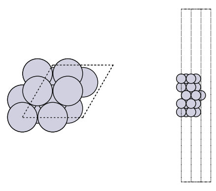

fig, axs = plt.subplots(1, 2)
plot_atoms(adslab, axs[0])
plot_atoms(adslab, axs[1], rotation=("-90x"))
axs[0].set_axis_off()
axs[1].set_axis_off()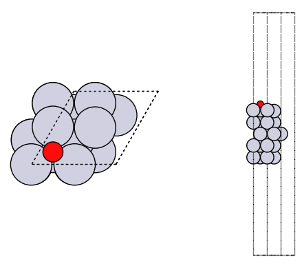

Molecular vibrations¶

from ase import Atoms
from ase.optimize import BFGS

predictor = pretrained_mlip.get_predict_unit("uma-s-1")
calc = FAIRChemCalculator(predictor, task_name="omol")

from ase.vibrations import Vibrations

n2 = Atoms("N2", [(0, 0, 0), (0, 0, 1.1)])
n2.info.update({"spin": 1, "charge": 0})
n2.calc = calc

BFGS(n2).run(fmax=0.01)

vib = Vibrations(n2)
vib.run()
vib.summary()

Bulk alloy phase behavior¶

Adapted from https://kitchingroup.cheme.cmu.edu/dft-book/dft.html#orgheadline29

We manually compute the formation energy of pure compounds and some alloy compositions to assess stability.

from ase.atoms import Atom, Atoms
from ase.filters import FrechetCellFilter
from ase.optimize import FIRE
from fairchem.core import FAIRChemCalculator, pretrained_mlip

predictor = pretrained_mlip.get_predict_unit("uma-s-1")

cu = Atoms(
    [Atom("Cu", [0.000, 0.000, 0.000])],
    cell=[[1.818, 0.000, 1.818], [1.818, 1.818, 0.000], [0.000, 1.818, 1.818]],
    pbc=True,
)
cu.calc = FAIRChemCalculator(predictor, task_name="omat")

opt = FIRE(FrechetCellFilter(cu))
opt.run(0.05, 100)

cu.get_potential_energy()

pd = Atoms(
    [Atom("Pd", [0.000, 0.000, 0.000])],
    cell=[[1.978, 0.000, 1.978], [1.978, 1.978, 0.000], [0.000, 1.978, 1.978]],
    pbc=True,
)
pd.calc = FAIRChemCalculator(predictor, task_name="omat")

opt = FIRE(FrechetCellFilter(pd))
opt.run(0.05, 100)

pd.get_potential_energy()

Alloy formation energies¶

cupd1 = Atoms(
    [Atom("Cu", [0.000, 0.000, 0.000]), Atom("Pd", [-1.652, 0.000, 2.039])],
    cell=[[0.000, -2.039, 2.039], [0.000, 2.039, 2.039], [-3.303, 0.000, 0.000]],
    pbc=True,
)  # Note pbc=True is important, it is not the default and OMAT

cupd1.calc = FAIRChemCalculator(predictor, task_name="omat")

opt = FIRE(FrechetCellFilter(cupd1))
opt.run(0.05, 100)

cupd1.get_potential_energy()

cupd2 = Atoms(
    [
        Atom("Cu", [-0.049, 0.049, 0.049]),
        Atom("Cu", [-11.170, 11.170, 11.170]),
        Atom("Pd", [-7.415, 7.415, 7.415]),
        Atom("Pd", [-3.804, 3.804, 3.804]),
    ],
    cell=[[-5.629, 3.701, 5.629], [-3.701, 5.629, 5.629], [-5.629, 5.629, 3.701]],
    pbc=True,
)
cupd2.calc = FAIRChemCalculator(predictor, task_name="omat")

opt = FIRE(FrechetCellFilter(cupd2))
opt.run(0.05, 100)

cupd2.get_potential_energy()

# Delta Hf cupd-1 = -0.11 eV/atom
hf1 = (
    cupd1.get_potential_energy() - cu.get_potential_energy() - pd.get_potential_energy()
)
hf1

# DFT: Delta Hf cupd-2 = -0.04 eV/atom
hf2 = (
    cupd2.get_potential_energy()
    - 2 * cu.get_potential_energy()
    - 2 * pd.get_potential_energy()
)
hf2

hf1 - hf2, (-0.11 - -0.04)

These indicate that cupd-1 and cupd-2 are both more stable than phase separated Cu and Pd, and that cupd-1 is more stable than cupd-2. The absolute formation energies differ from the DFT references, but the relative differences are quite close. The absolute differences could be due to DFT parameter choices (XC, psp, etc.).

Phonon calculation¶

This takes 4-10 minutes. Adapted from https://wiki.fysik.dtu.dk/ase/ase/phonons.html#example.

Phonons have applications in computing the stability and free energy of solids. See:

from ase.build import bulk
from ase.phonons import Phonons

predictor = pretrained_mlip.get_predict_unit("uma-s-1")
calc = FAIRChemCalculator(predictor, task_name="omat")

# Setup crystal
atoms = bulk("Al", "fcc", a=4.05)

# Phonon calculator
N = 7
ph = Phonons(atoms, calc, supercell=(N, N, N), delta=0.05)
ph.run()

# Read forces and assemble the dynamical matrix
ph.read(acoustic=True)
ph.clean()

path = atoms.cell.bandpath("GXULGK", npoints=100)
bs = ph.get_band_structure(path)

dos = ph.get_dos(kpts=(20, 20, 20)).sample_grid(npts=100, width=1e-3)

# Plot the band structure and DOS:
import matplotlib.pyplot as plt  # noqa

fig = plt.figure(figsize=(7, 4))
ax = fig.add_axes([0.12, 0.07, 0.67, 0.85])

emax = 0.04
bs.plot(ax=ax, emin=0.0, emax=emax)

dosax = fig.add_axes([0.8, 0.07, 0.17, 0.85])
dosax.fill_between(
    dos.get_weights(),
    dos.get_energies(),
    y2=0,
    color="grey",
    edgecolor="k",
    lw=1,
)

dosax.set_ylim(0, emax)
dosax.set_yticks([])
dosax.set_xticks([])
dosax.set_xlabel("DOS", fontsize=18);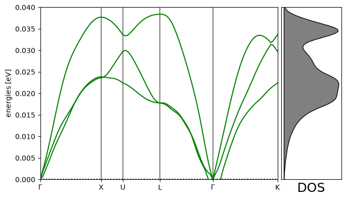

Transition States (NEBs)¶

Nudged elastic band calculations are among the most costly calculations we do. UMA makes these quicker!

We explore diffusion of an O adatom from an hcp to an fcc site on Pt(111).

Initial state¶

from ase.build import add_adsorbate, fcc111, molecule
from ase.optimize import LBFGS
from fairchem.core import FAIRChemCalculator, pretrained_mlip

predictor = pretrained_mlip.get_predict_unit("uma-s-1")
calc = FAIRChemCalculator(predictor, task_name="oc20")

# Set up your system as an ASE atoms object
initial = fcc111("Pt", (3, 3, 3), vacuum=8, periodic=True)

adsorbate = molecule("O")
add_adsorbate(initial, adsorbate, 2.0, "fcc")
initial.calc = calc

# Set up LBFGS dynamics object
opt = LBFGS(initial)
opt.run(0.05, 100)
print(initial.get_potential_energy())

Final state¶

# Set up your system as an ASE atoms object
final = fcc111("Pt", (3, 3, 3), vacuum=8, periodic=True)

adsorbate = molecule("O")
add_adsorbate(final, adsorbate, 2.0, "hcp")
final.calc = FAIRChemCalculator(predictor, task_name="oc20")

# Set up LBFGS dynamics object
opt = LBFGS(final)
opt.run(0.05, 100)
print(final.get_potential_energy())

Setup and relax the band¶

from ase.mep import NEB

images = [initial]
for i in range(3):
    image = initial.copy()
    image.calc = FAIRChemCalculator(predictor, task_name="oc20")
    images.append(image)

images.append(final)


neb = NEB(images)
neb.interpolate()

opt = LBFGS(neb, trajectory="neb.traj")
opt.run(0.05, 100)

from ase.mep import NEBTools

NEBTools(neb.images).plot_band();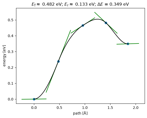

This could be a good initial guess to initialize an NEB in DFT.

Ideas for things you can do with UMA¶

Advanced applications¶

These take a while to run.

AdsorbML¶

It is so cheap to run these calculations that we can screen a broad range of adsorbate sites and rank them in stability. The AdsorbML approach automates this. This takes quite a while to run here, and we don’t do it in the workshop.

Expert adsorption energies¶

This tutorial reproduces Fig 6b from the following paper: Zhou, Jing, et al. “Enhanced Catalytic Activity of Bimetallic Ordered Catalysts for Nitrogen Reduction Reaction by Perturbation of Scaling Relations.” ACS Catalysis 134 (2023): 2190-2201 (Zhou et al. (2023)).

This takes up to an hour with a GPU, and much longer with a CPU.

CatTsunami¶

The CatTsunami tutorial is an example of enumerating initial and final states, and computing reaction paths between them with UMA.

Acknowledgments¶

This tutorial was originally compiled by John Kitchin (CMU) for the NAM29 catalysis tutorial session, using a variety of resources from the FAIR chemistry repository.

References¶

Musielewicz, J., Wang, X., Tian, T., & Ulissi, Z. (2022). FINETUNA: fine-tuning accelerated molecular simulations. Machine Learning: Science and Technology, 3(3), 03LT01. 10.1088/2632-2153/ac8fe0
Wang, X., Musielewicz, J., Tran, R., Kumar Ethirajan, S., Fu, X., Mera, H., Kitchin, J. R., Kurchin, R. C., & Ulissi, Z. W. (2024). Generalization of graph-based active learning relaxation strategies across materials. Machine Learning: Science and Technology, 5(2), 025018. 10.1088/2632-2153/ad37f0
Wander, B., Shuaibi, M., Kitchin, J. R., Ulissi, Z. W., & Zitnick, C. L. (2025). CatTSunami: Accelerating Transition State Energy Calculations with Pretrained Graph Neural Networks. ACS Catalysis, 15(7), 5283–5294. 10.1021/acscatal.4c04272
Wander, B., Musielewicz, J., Cheula, R., & Kitchin, J. R. (2025). Accessing Numerical Energy Hessians with Graph Neural Network Potentials and Their Application in Heterogeneous Catalysis. The Journal of Physical Chemistry C, 129(7), 3510–3521. 10.1021/acs.jpcc.4c07477
Zhou, J., Chen, X., Guo, M., Hu, W., Huang, B., & Yuan, D. (2023). Enhanced Catalytic Activity of Bimetallic Ordered Catalysts for Nitrogen Reduction Reaction by Perturbation of Scaling Relations. ACS Catalysis, 13(4), 2190–2201. 10.1021/acscatal.2c05877