Intro to adsorption energies#
To introduce OCP we start with using it to calculate adsorption energies for a simple, atomic adsorbate where we specify the site we want to the adsorption energy for. Conceptually, you do this like you would do it with density functional theory. You create a slab model for the surface, place an adsorbate on it as an initial guess, run a relaxation to get the lowest energy geometry, and then compute the adsorption energy using reference states for the adsorbate.
You do have to be careful in the details though. Some OCP model/checkpoint combinations return a total energy like density functional theory would, but some return an “adsorption energy” directly. You have to know which one you are using. In this example, the model we use returns an “adsorption energy”.
Intro to Adsorption energies#
Adsorption energies are always a reaction energy (an adsorbed species relative to some implied combination of reactants). There are many common schemes in the catalysis literature.
For example, you may want the adsorption energy of oxygen, and you might compute that from this reaction:
1/2 O2 + slab -> slab-O
DFT has known errors with the energy of a gas-phase O2 molecule, so it’s more common to compute this energy relative to a linear combination of H2O and H2. The suggested reference scheme for consistency with OC20 is a reaction
x CO + (x + y/2 - z) H2 + (z-x) H2O + w/2 N2 + * -> CxHyOzNw*
Here, x=y=w=0, z=1, so the reaction ends up as
-H2 + H2O + * -> O*
or alternatively,
H2O + * -> O* + H2
It is possible through thermodynamic cycles to compute other reactions. If we can look up rH1 below and compute rH2
H2 + 1/2 O2 -> H2O  re1 = -3.03 eV, from exp
H2O + * -> O* + H2  re2  # Get from UMA
Then, the adsorption energy for
1/2O2 + * -> O*
is just re1 + re2.
Based on https://atct.anl.gov/Thermochemical%20Data/version%201.118/species/?species_number=986, the formation energy of water is about -3.03 eV at standard state experimentally. You could also compute this using DFT, but you would probably get the wrong answer for this.
The first step is getting a checkpoint for the model we want to use. UMA is currently the state-of-the-art model and will provide total energy estimates at the RPBE level of theory if you use the “OC20” task.
Need to install fairchem-core or get UMA access or getting permissions/401 errors?
Install the necessary packages using pip, uv etc
Get access to any necessary huggingface gated models
Get and login to your Huggingface account
Request access to https://huggingface.co/facebook/UMA
Create a Huggingface token at https://huggingface.co/settings/tokens/ with the permission “Permissions: Read access to contents of all public gated repos you can access”
Add the token as an environment variable using
huggingface-cli loginor by setting the HF_TOKEN environment variable.
If you find your kernel is crashing, it probably means you have exceeded the allowed amount of memory. This checkpoint works fine in this example, but it may crash your kernel if you use it in the NRR example.
This next cell will automatically download the checkpoint from huggingface and load it.
from __future__ import annotations

from fairchem.core import FAIRChemCalculator, pretrained_mlip

predictor = pretrained_mlip.get_predict_unit("uma-s-1p1")
calc = FAIRChemCalculator(predictor, task_name="oc20")
WARNING:root:device was not explicitly set, using device='cuda'.
Next we can build a slab with an adsorbate on it. Here we use the ASE module to build a Pt slab. We use the experimental lattice constant that is the default. This can introduce some small errors with DFT since the lattice constant can differ by a few percent, and it is common to use DFT lattice constants. In this example, we do not constrain any layers.
from ase.build import add_adsorbate, fcc111
from ase.optimize import BFGS
# reference energies from a linear combination of H2O/N2/CO/H2!
atomic_reference_energies = {
    "H": -3.477,
    "N": -8.083,
    "O": -7.204,
    "C": -7.282,
}

re1 = -3.03

slab = fcc111("Pt", size=(2, 2, 5), vacuum=20.0)
slab.pbc = True

adslab = slab.copy()
add_adsorbate(adslab, "O", height=1.2, position="fcc")

slab.set_calculator(calc)
opt = BFGS(slab)
opt.run(fmax=0.05, steps=100)
slab_e = slab.get_potential_energy()

adslab.set_calculator(calc)
opt = BFGS(adslab)
opt.run(fmax=0.05, steps=100)
adslab_e = adslab.get_potential_energy()

# Energy for ((H2O-H2) + * -> *O) + (H2 + 1/2O2 -> H2) leads to 1/2O2 + * -> *O!
adslab_e - slab_e - atomic_reference_energies["O"] + re1
/tmp/ipykernel_5600/3752951811.py:17: FutureWarning: Please use atoms.calc = calc
  slab.set_calculator(calc)
      Step     Time          Energy          fmax
BFGS:    0 20:22:02     -104.695193        0.709590
BFGS:    1 20:22:02     -104.753187        0.607748
BFGS:    2 20:22:02     -104.906056        0.369388
BFGS:    3 20:22:02     -104.938753        0.439757
BFGS:    4 20:22:02     -105.016144        0.464014
BFGS:    5 20:22:03     -105.076560        0.356063
BFGS:    6 20:22:03     -105.112621        0.189413
BFGS:    7 20:22:03     -105.126757        0.045376
      Step     Time          Energy          fmax
BFGS:    0 20:22:03     -110.048788        1.757515
/tmp/ipykernel_5600/3752951811.py:22: FutureWarning: Please use atoms.calc = calc
  adslab.set_calculator(calc)
BFGS:    1 20:22:03     -110.230720        0.986276
BFGS:    2 20:22:03     -110.379353        0.731504
BFGS:    3 20:22:03     -110.430289        0.807337
BFGS:    4 20:22:03     -110.543669        0.692010
BFGS:    5 20:22:03     -110.617475        0.492775
BFGS:    6 20:22:03     -110.673456        0.666983
BFGS:    7 20:22:03     -110.721678        0.710539
BFGS:    8 20:22:03     -110.756903        0.443878
BFGS:    9 20:22:04     -110.769294        0.214535
BFGS:   10 20:22:04     -110.772451        0.091753
BFGS:   11 20:22:04     -110.772964        0.062467
BFGS:   12 20:22:04     -110.773259        0.046199
-1.4725024897882188
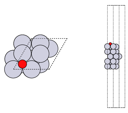
It is good practice to look at your geometries to make sure they are what you expect.
import matplotlib.pyplot as plt
from ase.visualize.plot import plot_atoms

fig, axs = plt.subplots(1, 2)
plot_atoms(slab, axs[0])
plot_atoms(slab, axs[1], rotation=("-90x"))
axs[0].set_axis_off()
axs[1].set_axis_off()

import matplotlib.pyplot as plt
from ase.visualize.plot import plot_atoms

fig, axs = plt.subplots(1, 2)
plot_atoms(adslab, axs[0])
plot_atoms(adslab, axs[1], rotation=("-90x"))
axs[0].set_axis_off()
axs[1].set_axis_off()
How did we do? We need a reference point. In the paper below, there is an atomic adsorption energy for O on Pt(111) of about -4.264 eV. This is for the reaction O + * -> O*. To convert this to the dissociative adsorption energy, we have to add the reaction:
1/2 O2 -> O D = 2.58 eV (expt)
to get a comparable energy of about -1.68 eV. There is about ~0.2 eV difference (we predicted -1.47 eV above, and the reference comparison is -1.68 eV) to account for. The biggest difference is likely due to the differences in exchange-correlation functional. The reference data used the PBE functional, and eSCN was trained on RPBE data. To additional places where there are differences include:
Difference in lattice constant
The reference energy used for the experiment references. These can differ by up to 0.5 eV from comparable DFT calculations.
How many layers are relaxed in the calculation
Some of these differences tend to be systematic, and you can calibrate and correct these, especially if you can augment these with your own DFT calculations.
See convergence study for some additional studies of factors that influence this number.
Exercises#
Explore the effect of the lattice constant on the adsorption energy.
Try different sites, including the bridge and top sites. Compare the energies, and inspect the resulting geometries.
Trends in adsorption energies across metals.#
Xu, Z., & Kitchin, J. R. (2014). Probing the coverage dependence of site and adsorbate configurational correlations on (111) surfaces of late transition metals. J. Phys. Chem. C, 118(44), 25597–25602. http://dx.doi.org/10.1021/jp508805h
These are atomic adsorption energies:
O + * -> O*
We have to do some work to get comparable numbers from OCP
H2 + 1/2 O2 -> H2O  re1 = -3.03 eV
H2O + * -> O* + H2  re2   # Get from UMA
O -> 1/2 O2         re3 = -2.58 eV
Then, the adsorption energy for
O + * -> O*
is just re1 + re2 + re3.
Here we just look at the fcc site on Pt. First, we get the data stored in the paper.
Next we get the structures and compute their energies. Some subtle points are that we have to account for stoichiometry, and normalize the adsorption energy by the number of oxygens.
First we get a reference energy from the paper (PBE, 0.25 ML O on Pt(111)).
import json

with open("energies.json") as f:
    edata = json.load(f)

with open("structures.json") as f:
    sdata = json.load(f)

edata["Pt"]["O"]["fcc"]["0.25"]
-4.263842000000002
Next, we load data from the SI to get the geometry to start from.
with open("structures.json") as f:
    s = json.load(f)

sfcc = s["Pt"]["O"]["fcc"]["0.25"]
Next, we construct the atomic geometry, run the geometry optimization, and compute the energy.
re3 = -2.58  # O -> 1/2 O2         re3 = -2.58 eV

from ase import Atoms

adslab = Atoms(sfcc["symbols"], positions=sfcc["pos"], cell=sfcc["cell"], pbc=True)

# Grab just the metal surface atoms
slab = adslab[adslab.arrays["numbers"] == adslab.arrays["numbers"][0]]
adsorbates = adslab[~(adslab.arrays["numbers"] == adslab.arrays["numbers"][0])]
slab.set_calculator(calc)
opt = BFGS(slab)
opt.run(fmax=0.05, steps=100)

adslab.set_calculator(calc)
opt = BFGS(adslab)

opt.run(fmax=0.05, steps=100)
re2 = (
    adslab.get_potential_energy()
    - slab.get_potential_energy()
    - sum([atomic_reference_energies[x] for x in adsorbates.get_chemical_symbols()])
)

nO = 0
for atom in adslab:
    if atom.symbol == "O":
        nO += 1
        re2 += re1 + re3

print(re2 / nO)
/tmp/ipykernel_5600/647904475.py:10: FutureWarning: Please use atoms.calc = calc
  slab.set_calculator(calc)
      Step     Time          Energy          fmax
BFGS:    0 20:22:06      -82.862062        1.000262
BFGS:    1 20:22:06      -82.918113        0.752920
BFGS:    2 20:22:06      -83.011695        0.335860
BFGS:    3 20:22:06      -83.016496        0.303120
BFGS:    4 20:22:06      -83.024496        0.224963
BFGS:    5 20:22:06      -83.030036        0.152567
BFGS:    6 20:22:07      -83.033360        0.088626
BFGS:    7 20:22:07      -83.034469        0.065747
BFGS:    8 20:22:07      -83.035208        0.068689
BFGS:    9 20:22:07      -83.035564        0.046754
      Step     Time          Energy          fmax
BFGS:    0 20:22:07      -88.770342        0.312348
BFGS:    1 20:22:07      -88.773631        0.271702
/tmp/ipykernel_5600/647904475.py:14: FutureWarning: Please use atoms.calc = calc
  adslab.set_calculator(calc)
BFGS:    2 20:22:07      -88.784474        0.104050
BFGS:    3 20:22:07      -88.786013        0.101458
BFGS:    4 20:22:07      -88.788552        0.106388
BFGS:    5 20:22:08      -88.790502        0.089090
BFGS:    6 20:22:08      -88.791972        0.096449
BFGS:    7 20:22:08      -88.792658        0.099419
BFGS:    8 20:22:08      -88.793178        0.077363
BFGS:    9 20:22:08      -88.793678        0.036094
-4.1641148097345075
Site correlations#
This cell reproduces a portion of a figure in the paper. We compare oxygen adsorption energies in the fcc and hcp sites across metals and coverages. These adsorption energies are highly correlated with each other because the adsorption sites are so similar.
At higher coverages, the agreement is not as good. This is likely because the model is extrapolating and needs to be fine-tuned.
import time

from tqdm import tqdm

t0 = time.time()

data = {"fcc": [], "hcp": []}

refdata = {"fcc": [], "hcp": []}


for metal in ["Cu", "Ag", "Pd", "Pt", "Rh", "Ir"]:
    print(metal)
    for site in ["fcc", "hcp"]:
        for adsorbate in ["O"]:
            for coverage in tqdm(["0.25"]):

                entry = s[metal][adsorbate][site][coverage]

                adslab = Atoms(
                    entry["symbols"],
                    positions=entry["pos"],
                    cell=entry["cell"],
                    pbc=True,
                )

                # Grab just the metal surface atoms
                adsorbates = adslab[
                    ~(adslab.arrays["numbers"] == adslab.arrays["numbers"][0])
                ]

                slab = adslab[adslab.arrays["numbers"] == adslab.arrays["numbers"][0]]
                slab.set_calculator(calc)
                opt = BFGS(slab)
                opt.run(fmax=0.05, steps=100)

                adslab.set_calculator(calc)
                opt = BFGS(adslab)
                opt.run(fmax=0.05, steps=100)

                re2 = (
                    adslab.get_potential_energy()
                    - slab.get_potential_energy()
                    - sum(
                        [
                            atomic_reference_energies[x]
                            for x in adsorbates.get_chemical_symbols()
                        ]
                    )
                )

                nO = 0
                for atom in adslab:
                    if atom.symbol == "O":
                        nO += 1
                        re2 += re1 + re3

                data[site] += [re2 / nO]
                refdata[site] += [edata[metal][adsorbate][site][coverage]]

f"Elapsed time = {time.time() - t0} seconds"
Cu
0%| | 0/1 [00:00<?, ?it/s]
      Step     Time          Energy          fmax
BFGS:    0 20:22:08      -48.910948        0.646351
BFGS:    1 20:22:08      -48.934031        0.539303
/tmp/ipykernel_5600/1356342052.py:33: FutureWarning: Please use atoms.calc = calc
  slab.set_calculator(calc)
BFGS: 2 20:22:08 -49.000044 0.280103
BFGS:    3 20:22:08      -49.002374        0.251321
BFGS:    4 20:22:08      -49.008810        0.158909
BFGS: 5 20:22:08 -49.013986 0.134401
BFGS:    6 20:22:09      -49.016868        0.071525
BFGS:    7 20:22:09      -49.017633        0.051269
BFGS: 8 20:22:09 -49.018011 0.047564
      Step     Time          Energy          fmax
BFGS:    0 20:22:09      -55.204221        0.339047
BFGS:    1 20:22:09      -55.206663        0.267938
/tmp/ipykernel_5600/1356342052.py:37: FutureWarning: Please use atoms.calc = calc
  adslab.set_calculator(calc)
BFGS: 2 20:22:09 -55.213712 0.160040
BFGS:    3 20:22:09      -55.215873        0.166183
BFGS:    4 20:22:09      -55.219674        0.116680
BFGS: 5 20:22:09 -55.221814 0.079418
BFGS:    6 20:22:09      -55.223360        0.075350
BFGS:    7 20:22:09      -55.224365        0.090298
BFGS: 8 20:22:09 -55.225517 0.098885
BFGS:    9 20:22:10      -55.226530        0.068547
BFGS:   10 20:22:10      -55.226977        0.043001
100%|██████████| 1/1 [00:01<00:00, 1.75s/it]
100%|██████████| 1/1 [00:01<00:00, 1.75s/it]
0%| | 0/1 [00:00<?, ?it/s]
      Step     Time          Energy          fmax
BFGS:    0 20:22:10      -48.936503        0.552695
BFGS:    1 20:22:10      -48.954084        0.470533
BFGS:    2 20:22:10      -49.008576        0.210998
BFGS:    3 20:22:10      -49.009768        0.197685
BFGS:    4 20:22:10      -49.017746        0.041126
      Step     Time          Energy          fmax
BFGS:    0 20:22:10      -55.119070        0.305598
BFGS:    1 20:22:10      -55.120918        0.239016
BFGS:    2 20:22:10      -55.125705        0.129128
BFGS:    3 20:22:10      -55.127340        0.147616
BFGS:    4 20:22:11      -55.130397        0.128628
BFGS:    5 20:22:11      -55.132308        0.103155
BFGS:    6 20:22:11      -55.133381        0.051684
BFGS:    7 20:22:11      -55.133851        0.056041
BFGS:    8 20:22:11      -55.134358        0.071230
BFGS:    9 20:22:11      -55.135043        0.069440
100%|██████████| 1/1 [00:01<00:00, 1.41s/it]
100%|██████████| 1/1 [00:01<00:00, 1.41s/it]
BFGS:   10 20:22:11      -55.135574        0.039939
Ag
0%| | 0/1 [00:00<?, ?it/s]
      Step     Time          Energy          fmax
BFGS:    0 20:22:11      -33.034314        0.634820
BFGS:    1 20:22:11      -33.053470        0.551048
BFGS:    2 20:22:11      -33.120905        0.172022
BFGS: 3 20:22:11 -33.122778 0.157330
BFGS:    4 20:22:12      -33.124181        0.143386
BFGS:    5 20:22:12      -33.126943        0.112458
BFGS: 6 20:22:12 -33.130771 0.110654
BFGS:    7 20:22:12      -33.133994        0.067525
BFGS:    8 20:22:12      -33.134835        0.034888
      Step     Time          Energy          fmax
BFGS:    0 20:22:12      -38.173509        0.098015
BFGS:    1 20:22:12      -38.174435        0.094365
BFGS:    2 20:22:12      -38.184907        0.084030
BFGS: 3 20:22:12 -38.185732 0.085432
BFGS:    4 20:22:12      -38.189035        0.086087
BFGS:    5 20:22:12      -38.190952        0.068846
BFGS: 6 20:22:12 -38.192257 0.087460
BFGS:    7 20:22:13      -38.193187        0.076900
BFGS:    8 20:22:13      -38.193674        0.042580
100%|██████████| 1/1 [00:01<00:00, 1.57s/it]
100%|██████████| 1/1 [00:01<00:00, 1.57s/it]
0%| | 0/1 [00:00<?, ?it/s]
      Step     Time          Energy          fmax
BFGS:    0 20:22:13      -33.056750        0.557366
BFGS:    1 20:22:13      -33.071228        0.489412
BFGS:    2 20:22:13      -33.126397        0.123825
BFGS:    3 20:22:13      -33.127308        0.112960
BFGS:    4 20:22:13      -33.128516        0.097373
BFGS:    5 20:22:13      -33.130260        0.079535
BFGS:    6 20:22:13      -33.133160        0.076344
BFGS:    7 20:22:13      -33.134742        0.040732
      Step     Time          Energy          fmax
BFGS:    0 20:22:13      -38.102026        0.092717
BFGS:    1 20:22:13      -38.102856        0.088836
BFGS:    2 20:22:14      -38.111088        0.134657
BFGS:    3 20:22:14      -38.112011        0.120324
BFGS:    4 20:22:14      -38.115289        0.063997
BFGS:    5 20:22:14      -38.116155        0.056403
BFGS:    6 20:22:14      -38.116711        0.058196
BFGS:    7 20:22:14      -38.117579        0.073181
BFGS:    8 20:22:14      -38.118452        0.057890
BFGS:    9 20:22:14      -38.118833        0.026042
100%|██████████| 1/1 [00:01<00:00, 1.57s/it]
100%|██████████| 1/1 [00:01<00:00, 1.57s/it]
Pd
0%| | 0/1 [00:00<?, ?it/s]
      Step     Time          Energy          fmax
BFGS:    0 20:22:14      -70.165062        0.631446
BFGS:    1 20:22:14      -70.189910        0.508128
BFGS: 2 20:22:14 -70.241649 0.191934
BFGS:    3 20:22:15      -70.243347        0.182565
BFGS:    4 20:22:15      -70.248575        0.144558
BFGS: 5 20:22:15 -70.251930 0.115933
BFGS:    6 20:22:15      -70.254308        0.074837
BFGS:    7 20:22:15      -70.255205        0.059447
BFGS: 8 20:22:15 -70.255944 0.041110
      Step     Time          Energy          fmax
BFGS:    0 20:22:15      -76.130241        0.213656
BFGS:    1 20:22:15      -76.133242        0.190305
BFGS: 2 20:22:15 -76.148718 0.169626
BFGS:    3 20:22:15      -76.150813        0.152251
BFGS:    4 20:22:15      -76.154313        0.130512
BFGS: 5 20:22:15 -76.157057 0.106146
BFGS:    6 20:22:16      -76.159303        0.088117
BFGS:    7 20:22:16      -76.160431        0.080496
BFGS: 8 20:22:16 -76.161131 0.064485
100%|██████████| 1/1 [00:01<00:00, 1.65s/it]
100%|██████████| 1/1 [00:01<00:00, 1.66s/it]
BFGS: 9 20:22:16 -76.161613 0.043008
0%| | 0/1 [00:00<?, ?it/s]
      Step     Time          Energy          fmax
BFGS:    0 20:22:16      -70.197711        0.454636
BFGS:    1 20:22:16      -70.211775        0.373893
BFGS:    2 20:22:16      -70.245977        0.178178
BFGS: 3 20:22:16 -70.247163 0.164572
BFGS:    4 20:22:16      -70.253348        0.078706
BFGS:    5 20:22:16      -70.254511        0.075507
BFGS: 6 20:22:16 -70.255271 0.058127
BFGS:    7 20:22:17      -70.255844        0.036952
      Step     Time          Energy          fmax
BFGS:    0 20:22:17      -75.892387        0.169440
BFGS: 1 20:22:17 -75.895234 0.150799
BFGS:    2 20:22:17      -75.906632        0.144107
BFGS:    3 20:22:17      -75.908424        0.135658
BFGS: 4 20:22:17 -75.912428 0.129018
BFGS:    5 20:22:17      -75.915496        0.108687
BFGS:    6 20:22:17      -75.917928        0.075296
BFGS: 7 20:22:17 -75.918956 0.067268
100%|██████████| 1/1 [00:01<00:00, 1.49s/it]
100%|██████████| 1/1 [00:01<00:00, 1.49s/it]
BFGS:    8 20:22:17      -75.919479        0.044584
Pt
0%| | 0/1 [00:00<?, ?it/s]
      Step     Time          Energy          fmax
BFGS:    0 20:22:17      -82.862063        1.000262
BFGS:    1 20:22:18      -82.918113        0.752920
BFGS:    2 20:22:18      -83.011694        0.335860
BFGS: 3 20:22:18 -83.016496 0.303120
BFGS:    4 20:22:18      -83.024497        0.224963
BFGS:    5 20:22:18      -83.030036        0.152567
BFGS: 6 20:22:18 -83.033361 0.088626
BFGS:    7 20:22:18      -83.034469        0.065746
BFGS:    8 20:22:18      -83.035208        0.068691
BFGS: 9 20:22:18 -83.035563 0.046754
      Step     Time          Energy          fmax
BFGS:    0 20:22:18      -88.770343        0.312349
BFGS:    1 20:22:18      -88.773631        0.271703
BFGS: 2 20:22:18 -88.784473 0.104050
BFGS:    3 20:22:19      -88.786014        0.101458
BFGS:    4 20:22:19      -88.788552        0.106393
BFGS: 5 20:22:19 -88.790502 0.089090
BFGS:    6 20:22:19      -88.791971        0.096441
BFGS:    7 20:22:19      -88.792659        0.099420
BFGS: 8 20:22:19 -88.793180 0.077367
100%|██████████| 1/1 [00:01<00:00, 1.74s/it]
100%|██████████| 1/1 [00:01<00:00, 1.74s/it]
BFGS: 9 20:22:19 -88.793679 0.036096
0%| | 0/1 [00:00<?, ?it/s]
      Step     Time          Energy          fmax
BFGS:    0 20:22:19      -82.946997        0.675644
BFGS:    1 20:22:19      -82.973149        0.546704
BFGS:    2 20:22:19      -83.026506        0.203005
BFGS: 3 20:22:19 -83.028070 0.183991
BFGS:    4 20:22:20      -83.033698        0.083392
BFGS:    5 20:22:20      -83.034396        0.061068
BFGS: 6 20:22:20 -83.035121 0.048400
      Step     Time          Energy          fmax
BFGS:    0 20:22:20      -88.350562        0.234982
BFGS:    1 20:22:20      -88.353606        0.203898
BFGS: 2 20:22:20 -88.362976 0.117094
BFGS:    3 20:22:20      -88.364342        0.121252
BFGS:    4 20:22:20      -88.368499        0.090134
BFGS: 5 20:22:20 -88.370482 0.073281
BFGS:    6 20:22:20      -88.371786        0.075217
BFGS:    7 20:22:20      -88.372317        0.079580
BFGS: 8 20:22:20 -88.372730 0.061426
100%|██████████| 1/1 [00:01<00:00, 1.50s/it]
100%|██████████| 1/1 [00:01<00:00, 1.50s/it]
BFGS:    9 20:22:21      -88.373020        0.027209
Rh
0%| | 0/1 [00:00<?, ?it/s]
      Step     Time          Energy          fmax
BFGS:    0 20:22:21     -100.192566        0.688933
BFGS:    1 20:22:21     -100.218240        0.600213
BFGS:    2 20:22:21     -100.286833        0.174739
BFGS: 3 20:22:21 -100.289768 0.129381
BFGS:    4 20:22:21     -100.298132        0.066639
BFGS:    5 20:22:21     -100.299264        0.053478
BFGS: 6 20:22:21 -100.299777 0.045082
      Step     Time          Energy          fmax
BFGS:    0 20:22:21     -106.921794        0.203149
BFGS:    1 20:22:21     -106.924541        0.168907
BFGS: 2 20:22:21 -106.930976 0.052441
100%|██████████| 1/1 [00:00<00:00, 1.00it/s]
100%|██████████| 1/1 [00:00<00:00, 1.00it/s]
BFGS: 3 20:22:22 -106.931584 0.045559
0%| | 0/1 [00:00<?, ?it/s]
      Step     Time          Energy          fmax
BFGS:    0 20:22:22     -100.171740        0.714774
BFGS:    1 20:22:22     -100.203866        0.626030
BFGS:    2 20:22:22     -100.287845        0.263192
BFGS: 3 20:22:22 -100.290543 0.195973
BFGS:    4 20:22:22     -100.297165        0.080364
BFGS:    5 20:22:22     -100.299033        0.056460
BFGS: 6 20:22:22 -100.299773 0.043868
      Step     Time          Energy          fmax
BFGS:    0 20:22:22     -106.876840        0.168839
BFGS:    1 20:22:22     -106.879420        0.139489
BFGS: 2 20:22:22 -106.885549 0.071255
BFGS:    3 20:22:23     -106.886238        0.064286
BFGS:    4 20:22:23     -106.886580        0.054980
BFGS: 5 20:22:23 -106.886841 0.043052
100%|██████████| 1/1 [00:01<00:00, 1.17s/it]
100%|██████████| 1/1 [00:01<00:00, 1.17s/it]
Ir
0%| | 0/1 [00:00<?, ?it/s]
      Step     Time          Energy          fmax
BFGS:    0 20:22:23     -124.235610        1.189926
BFGS: 1 20:22:23 -124.310841 0.937183
BFGS: 2 20:22:23 -124.422189 0.140826
BFGS: 3 20:22:23 -124.425270 0.133780
BFGS: 4 20:22:23 -124.429598 0.060640
BFGS: 5 20:22:23 -124.430258 0.038670
      Step     Time          Energy          fmax
BFGS:    0 20:22:23     -130.605624        0.371645
BFGS: 1 20:22:23 -130.616146 0.265890
BFGS: 2 20:22:24 -130.630316 0.110764
BFGS: 3 20:22:24 -130.633616 0.094356
BFGS: 4 20:22:24 -130.634275 0.075694
BFGS: 5 20:22:24 -130.634990 0.065695
BFGS: 6 20:22:24 -130.636199 0.083031
BFGS: 7 20:22:24 -130.636656 0.075132
BFGS: 8 20:22:24 -130.637048 0.047436
100%|██████████| 1/1 [00:01<00:00, 1.33s/it]
100%|██████████| 1/1 [00:01<00:00, 1.33s/it]
0%| | 0/1 [00:00<?, ?it/s]
      Step     Time          Energy          fmax
BFGS:    0 20:22:24     -124.227592        1.165685
BFGS:    1 20:22:24     -124.311476        0.915619
BFGS:    2 20:22:24     -124.422556        0.165136
BFGS: 3 20:22:24 -124.425477 0.200268
BFGS:    4 20:22:25     -124.428763        0.168861
BFGS:    5 20:22:25     -124.430255        0.088395
BFGS: 6 20:22:25 -124.430559 0.041798
      Step     Time          Energy          fmax
BFGS:    0 20:22:25     -130.496158        0.405482
BFGS:    1 20:22:25     -130.507202        0.266991
BFGS: 2 20:22:25 -130.518616 0.126414
BFGS:    3 20:22:25     -130.522315        0.080268
BFGS:    4 20:22:25     -130.523181        0.066553
BFGS: 5 20:22:25 -130.523452 0.056611
BFGS:    6 20:22:25     -130.524510        0.055662
BFGS:    7 20:22:25     -130.524679        0.042700
100%|██████████| 1/1 [00:01<00:00, 1.33s/it]
100%|██████████| 1/1 [00:01<00:00, 1.33s/it]
'Elapsed time = 17.53719186782837 seconds'
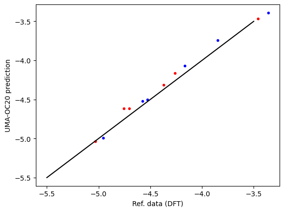
First, we compare the computed data and reference data. There is a systematic difference of about 0.5 eV due to the difference between RPBE and PBE functionals, and other subtle differences like lattice constant differences and reference energy differences. This is pretty typical, and an expected deviation.
plt.plot(refdata["fcc"], data["fcc"], "r.", label="fcc")
plt.plot(refdata["hcp"], data["hcp"], "b.", label="hcp")
plt.plot([-5.5, -3.5], [-5.5, -3.5], "k-")
plt.xlabel("Ref. data (DFT)")
plt.ylabel("UMA-OC20 prediction");
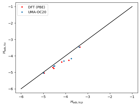
Next we compare the correlation between the hcp and fcc sites. Here we see the same trends. The data falls below the parity line because the hcp sites tend to be a little weaker binding than the fcc sites.
plt.plot(refdata["hcp"], refdata["fcc"], "r.")
plt.plot(data["hcp"], data["fcc"], ".")
plt.plot([-6, -1], [-6, -1], "k-")
plt.xlabel("$H_{ads, hcp}$")
plt.ylabel("$H_{ads, fcc}$")
plt.legend(["DFT (PBE)", "UMA-OC20"]);
Exercises#
You can also explore a few other adsorbates: C, H, N.
Explore the higher coverages. The deviations from the reference data are expected to be higher, but relative differences tend to be better. You probably need fine tuning to improve this performance. This data set doesn’t have forces though, so it isn’t practical to do it here.
Next steps#
In the next step, we consider some more complex adsorbates in nitrogen reduction, and how we can leverage OCP to automate the search for the most stable adsorbate geometry. See the next step.
Convergence study#
In Calculating adsorption energies we discussed some possible reasons we might see a discrepancy. Here we investigate some factors that impact the computed energies.
In this section, the energies refer to the reaction 1/2 O2 -> O*.
Effects of number of layers#
Slab thickness could be a factor. Here we relax the whole slab, and see by about 4 layers the energy is converged to ~0.02 eV.
for nlayers in [3, 4, 5, 6, 7, 8]:
    slab = fcc111("Pt", size=(2, 2, nlayers), vacuum=10.0)

    slab.pbc = True
    slab.set_calculator(calc)
    opt_slab = BFGS(slab, logfile=None)
    opt_slab.run(fmax=0.05, steps=100)
    slab_e = slab.get_potential_energy()

    adslab = slab.copy()
    add_adsorbate(adslab, "O", height=1.2, position="fcc")

    adslab.pbc = True
    adslab.set_calculator(calc)
    opt_adslab = BFGS(adslab, logfile=None)
    opt_adslab.run(fmax=0.05, steps=100)
    adslab_e = adslab.get_potential_energy()

    print(
        f"nlayers = {nlayers}: {adslab_e - slab_e - atomic_reference_energies['O'] + re1:1.2f} eV"
    )
/tmp/ipykernel_5600/338101817.py:5: FutureWarning: Please use atoms.calc = calc
  slab.set_calculator(calc)
/tmp/ipykernel_5600/338101817.py:14: FutureWarning: Please use atoms.calc = calc
  adslab.set_calculator(calc)
nlayers = 3: -1.58 eV
nlayers = 4: -1.47 eV
nlayers = 5: -1.47 eV
nlayers = 6: -1.46 eV
nlayers = 7: -1.47 eV
nlayers = 8: -1.47 eV
Effects of relaxation#
It is common to only relax a few layers, and constrain lower layers to bulk coordinates. We do that here. We only relax the adsorbate and the top layer.
This has a small effect (0.1 eV).
from ase.constraints import FixAtoms

for nlayers in [3, 4, 5, 6, 7, 8]:
    slab = fcc111("Pt", size=(2, 2, nlayers), vacuum=10.0)

    slab.set_constraint(FixAtoms(mask=[atom.tag > 1 for atom in slab]))
    slab.pbc = True
    slab.set_calculator(calc)
    opt_slab = BFGS(slab, logfile=None)
    opt_slab.run(fmax=0.05, steps=100)
    slab_e = slab.get_potential_energy()

    adslab = slab.copy()
    add_adsorbate(adslab, "O", height=1.2, position="fcc")

    adslab.set_constraint(FixAtoms(mask=[atom.tag > 1 for atom in adslab]))
    adslab.pbc = True
    adslab.set_calculator(calc)
    opt_adslab = BFGS(adslab, logfile=None)
    opt_adslab.run(fmax=0.05, steps=100)
    adslab_e = adslab.get_potential_energy()

    print(
        f"nlayers = {nlayers}: {adslab_e - slab_e - atomic_reference_energies['O'] + re1:1.2f} eV"
    )
/tmp/ipykernel_5600/1426773950.py:8: FutureWarning: Please use atoms.calc = calc
  slab.set_calculator(calc)
/tmp/ipykernel_5600/1426773950.py:18: FutureWarning: Please use atoms.calc = calc
  adslab.set_calculator(calc)
nlayers = 3: -1.47 eV
nlayers = 4: -1.35 eV
nlayers = 5: -1.35 eV
nlayers = 6: -1.34 eV
nlayers = 7: -1.35 eV
nlayers = 8: -1.35 eV
Unit cell size#
Coverage effects are quite noticeable with oxygen. Here we consider larger unit cells. This effect is large, and the results don’t look right, usually adsorption energies get more favorable at lower coverage, not less. This suggests fine-tuning could be important even at low coverages.
for size in [1, 2, 3, 4, 5]:

    slab = fcc111("Pt", size=(size, size, 5), vacuum=10.0)

    slab.set_constraint(FixAtoms(mask=[atom.tag > 1 for atom in slab]))
    slab.pbc = True
    slab.set_calculator(calc)
    opt_slab = BFGS(slab, logfile=None)
    opt_slab.run(fmax=0.05, steps=100)
    slab_e = slab.get_potential_energy()

    adslab = slab.copy()
    add_adsorbate(adslab, "O", height=1.2, position="fcc")

    adslab.set_constraint(FixAtoms(mask=[atom.tag > 1 for atom in adslab]))
    adslab.pbc = True
    adslab.set_calculator(calc)
    opt_adslab = BFGS(adslab, logfile=None)
    opt_adslab.run(fmax=0.05, steps=100)
    adslab_e = adslab.get_potential_energy()

    print(
        f"({size}x{size}): {adslab_e - slab_e - atomic_reference_energies['O'] + re1:1.2f} eV"
    )
/tmp/ipykernel_5600/3371624330.py:7: FutureWarning: Please use atoms.calc = calc
  slab.set_calculator(calc)
/tmp/ipykernel_5600/3371624330.py:17: FutureWarning: Please use atoms.calc = calc
  adslab.set_calculator(calc)
(1x1): -0.12 eV
(2x2): -1.35 eV
(3x3): -1.38 eV
(4x4): -1.41 eV
(5x5): -1.42 eV
Summary#
As with DFT, you should take care to see how these kinds of decisions affect your results, and determine if they would change any interpretations or not.