UMA Intro Tutorial#
This tutorial will walk you through a few examples of how you can use UMA. Each step is covered in more detail elsewhere in the documentation, but this is well suited to a ~1-2 hour tutorial session for researchers new to UMA but with some background in ASE and molecular simulations.
Before you start / installation#
You need to get a HuggingFace account and request access to the UMA models.
You need a Huggingface account, request access to https://huggingface.co/facebook/UMA, and to create a Huggingface token at https://huggingface.co/settings/tokens/ with these permission:
Permissions: Read access to contents of all public gated repos you can access
Then, add the token as an environment variable (using huggingface-cli login:
# Enter token via huggingface-cli
! huggingface-cli login
or you can set the token via HF_TOKEN variable:
# Set token via env variable
import os
os.environ['HF_TOKEN'] = 'MYTOKEN'
Installation process#
It may be enough to use pip install fairchem-core. This gets you the latest version on PyPi (https://pypi.org/project/fairchem-core/)
Here we install some sub-packages. This can take 2-5 minutes to run.
! pip install fairchem-core fairchem-data-oc fairchem-applications-cattsunami x3dase
# Check that packages are installed
!pip list | grep fairchem
fairchem-applications-cattsunami   1.1.2.dev148+g4c07b0a8
fairchem-core                      2.13.1.dev26+g4c07b0a8
fairchem-data-oc                   1.0.3.dev148+g4c07b0a8
fairchem-data-omat                 0.2.1.dev53+g4c07b0a8
import fairchem.core

fairchem.core.__version__
'2.13.1.dev26+g4c07b0a8'
Illustrative examples#
These should just run, and are here to show some basic uses.
Critical points:
Create a calculator
Specify the task_name
Use calculator like other ASE calculators
Spin gap energy - OMOL#
This is the difference in energy between a triplet and single ground state for a CH2 radical. This downloads a ~1GB checkpoint the first time you run it.
We don’t set a device here, so we get a warning about using a CPU device. You can ignore that. If a CUDA environment is available, a GPU may be used to speed up the calculations.
from fairchem.core import FAIRChemCalculator, pretrained_mlip

predictor = pretrained_mlip.get_predict_unit("uma-s-1")
WARNING:root:device was not explicitly set, using device='cuda'.
from ase.build import molecule

#  singlet CH2
singlet = molecule("CH2_s1A1d")
singlet.info.update({"spin": 1, "charge": 0})
singlet.calc = FAIRChemCalculator(predictor, task_name="omol")

#  triplet CH2
triplet = molecule("CH2_s3B1d")
triplet.info.update({"spin": 3, "charge": 0})
triplet.calc = FAIRChemCalculator(predictor, task_name="omol")

print(triplet.get_potential_energy() - singlet.get_potential_energy())
-0.5508372783660889
Example of adsorbate relaxation - OC20#
Here we just setup a Cu(100) slab with a CO on it and relax it.
This is an OC20 task because it is a slab with an adsorbate.
We specify an explicit device in the predictor here, and avoid the warning.
from ase.build import add_adsorbate, fcc100, molecule
from ase.optimize import LBFGS
from fairchem.core import FAIRChemCalculator, pretrained_mlip

predictor = pretrained_mlip.get_predict_unit("uma-s-1")
calc = FAIRChemCalculator(predictor, task_name="oc20")

# Set up your system as an ASE atoms object
slab = fcc100("Cu", (3, 3, 3), vacuum=8, periodic=True)

adsorbate = molecule("CO")
add_adsorbate(slab, adsorbate, 2.0, "bridge")
slab.calc = calc

# Set up LBFGS dynamics object
opt = LBFGS(slab)
opt.run(0.05, 100)
print(slab.get_potential_energy())
WARNING:root:device was not explicitly set, using device='cuda'.
       Step     Time          Energy          fmax
LBFGS:    0 21:52:21      -89.596203       11.451670
LBFGS:    1 21:52:22      -92.497568        6.543859
LBFGS:    2 21:52:22      -92.624428        7.536283
LBFGS:    3 21:52:22      -93.000906        3.715973
LBFGS:    4 21:52:22      -93.158687        3.479858
LBFGS:    5 21:52:22      -93.264149        2.256852
LBFGS:    6 21:52:22      -93.505251        1.133162
LBFGS:    7 21:52:22      -93.595938        0.991849
LBFGS:    8 21:52:22      -93.705356        0.683693
LBFGS:    9 21:52:22      -93.791545        0.506521
LBFGS:   10 21:52:22      -93.837927        0.364016
LBFGS:   11 21:52:22      -93.856805        0.349534
LBFGS:   12 21:52:22      -93.881769        0.498560
LBFGS:   13 21:52:23      -93.900197        0.432910
LBFGS:   14 21:52:23      -93.910015        0.156405
LBFGS:   15 21:52:23      -93.915885        0.170004
LBFGS:   16 21:52:23      -93.922146        0.211723
LBFGS:   17 21:52:23      -93.929011        0.260897
LBFGS:   18 21:52:23      -93.935161        0.183900
LBFGS:   19 21:52:23      -93.938071        0.057366
LBFGS:   20 21:52:23      -93.938498        0.039144
-93.9384984000145
Example bulk relaxation - OMAT#
from ase.build import bulk
from ase.filters import FrechetCellFilter
from ase.optimize import FIRE
from fairchem.core import FAIRChemCalculator, pretrained_mlip

predictor = pretrained_mlip.get_predict_unit("uma-s-1")
calc = FAIRChemCalculator(predictor, task_name="omat")

atoms = bulk("Fe")
atoms.calc = calc

opt = FIRE(FrechetCellFilter(atoms))
opt.run(0.05, 100)

print(atoms.get_stress())  # !!!! We get stress now!
WARNING:root:device was not explicitly set, using device='cuda'.
      Step     Time          Energy          fmax
FIRE:    0 21:52:25       -8.261158        0.651784
FIRE:    1 21:52:26       -8.271310        0.358119
FIRE:    2 21:52:26       -8.264588        1.650196
FIRE:    3 21:52:26       -8.273672        0.177966
FIRE:    4 21:52:26       -8.272634        0.269087
FIRE:    5 21:52:26       -8.272766        0.257552
FIRE:    6 21:52:26       -8.273009        0.234351
FIRE:    7 21:52:26       -8.273319        0.199206
FIRE:    8 21:52:26       -8.273635        0.151744
FIRE:    9 21:52:26       -8.273890        0.091454
FIRE:   10 21:52:26       -8.274015        0.017801
[1.5562563e-03 1.5562196e-03 1.5562959e-03 3.4555761e-08 3.1117042e-09
 3.7002938e-08]
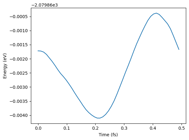
Molecular dynamics - OMOL#
import matplotlib.pyplot as plt

from ase import units
from ase.build import molecule
from ase.io import Trajectory
from ase.md.langevin import Langevin
from fairchem.core import FAIRChemCalculator, pretrained_mlip

predictor = pretrained_mlip.get_predict_unit("uma-s-1")
calc = FAIRChemCalculator(predictor, task_name="omol")

atoms = molecule("H2O")
atoms.info.update(charge=0, spin=1)  # For omol

atoms.calc = calc

dyn = Langevin(
    atoms,
    timestep=0.1 * units.fs,
    temperature_K=400,
    friction=0.001 / units.fs,
)

trajectory = Trajectory("my_md.traj", "w", atoms)
dyn.attach(trajectory.write, interval=1)
dyn.run(steps=50)

# See some results - not paper ready!
traj = Trajectory("my_md.traj")
plt.plot(
    [i * 0.1 * units.fs for i in range(len(traj))],
    [a.get_potential_energy() for a in traj],
)
plt.xlabel("Time (fs)")
plt.ylabel("Energy (eV)");
WARNING:root:device was not explicitly set, using device='cuda'.
Catalyst Adsorption energies#
The basic approach in computing an adsorption energy is to compute this energy difference:
dH = E_adslab - E_slab - E_ads
We use UMA for two of these energies E_adslab and E_slab. For E_ads We have to do something a little different. The OC20 task is not trained for molecules or molecular fragments. We use atomic energy reference energies instead. These are tabulated below.
The OC20 reference scheme is this reaction:
x CO + (x + y/2 - z) H2 + (z-x) H2O + w/2 N2 + * -> CxHyOzNw*
For this example we have
-H2 + H2O + * -> O*. "O": -7.204 eV
Where "O": -7.204 is a constant.
To get the desired reaction energy we want we add the formation energy of water. We use either DFT or experimental values for this reaction energy.
1/2O2 + H2 -> H2O
Alternatives to this approach are using DFT to estimate the energy of 1/2 O2, just make sure to use consistent settings with your task. You should not use OMOL for this.
from ase.build import add_adsorbate, fcc111
from ase.optimize import BFGS
from fairchem.core import FAIRChemCalculator, pretrained_mlip

predictor = pretrained_mlip.get_predict_unit("uma-s-1")
calc = FAIRChemCalculator(predictor, task_name="oc20")
WARNING:root:device was not explicitly set, using device='cuda'.
# reference energies from a linear combination of H2O/N2/CO/H2!
atomic_reference_energies = {
    "H": -3.477,
    "N": -8.083,
    "O": -7.204,
    "C": -7.282,
}

re1 = -3.03  # Water formation energy from experiment

slab = fcc111("Pt", size=(2, 2, 5), vacuum=20.0)
slab.pbc = True

adslab = slab.copy()
add_adsorbate(adslab, "O", height=1.2, position="fcc")

slab.calc = calc
opt = BFGS(slab)
print("Relaxing slab")
opt.run(fmax=0.05, steps=100)
slab_e = slab.get_potential_energy()

adslab.calc = calc
opt = BFGS(adslab)
print("\nRelaxing adslab")
opt.run(fmax=0.05, steps=100)
adslab_e = adslab.get_potential_energy()
Relaxing slab
      Step     Time          Energy          fmax
BFGS:    0 21:52:35     -104.710392        0.707696
BFGS:    1 21:52:35     -104.767890        0.605448
BFGS:    2 21:52:35     -104.919425        0.369265
BFGS:    3 21:52:35     -104.952877        0.441349
BFGS:    4 21:52:35     -105.030000        0.467592
BFGS:    5 21:52:35     -105.091451        0.365231
BFGS:    6 21:52:35     -105.128721        0.195037
BFGS:    7 21:52:36     -105.143315        0.048836

Relaxing adslab
      Step     Time          Energy          fmax
BFGS:    0 21:52:36     -110.055657        1.762239
BFGS:    1 21:52:36     -110.239039        0.996808
BFGS:    2 21:52:36     -110.389562        0.747533
BFGS:    3 21:52:36     -110.441196        0.818361
BFGS:    4 21:52:36     -110.557367        0.688425
BFGS:    5 21:52:36     -110.631217        0.497350
BFGS:    6 21:52:36     -110.687290        0.690799
BFGS:    7 21:52:36     -110.737889        0.729393
BFGS:    8 21:52:36     -110.774873        0.435709
BFGS:    9 21:52:36     -110.786666        0.199874
BFGS:   10 21:52:36     -110.789560        0.080701
BFGS:   11 21:52:36     -110.790040        0.057997
BFGS:   12 21:52:37     -110.790287        0.044009
Now we compute the adsorption energy.
# Energy for ((H2O-H2) + * -> *O) + (H2 + 1/2O2 -> H2O) leads to 1/2O2 + * -> *O!
adslab_e - slab_e - atomic_reference_energies["O"] + re1
-1.4729712207147325
How did we do? We need a reference point. In the paper below, there is an atomic adsorption energy for O on Pt(111) of about -4.264 eV. This is for the reaction O + * -> O*. To convert this to the dissociative adsorption energy, we have to add the reaction:
1/2 O2 -> O D = 2.58 eV (expt)
to get a comparable energy of about -1.68 eV. There is about ~0.2 eV difference (we predicted -1.47 eV above, and the reference comparison is -1.68 eV) to account for. The biggest difference is likely due to the differences in exchange-correlation functional. The reference data used the PBE functional, and eSCN was trained on RPBE data. To additional places where there are differences include:
Difference in lattice constant
The reference energy used for the experiment references. These can differ by up to 0.5 eV from comparable DFT calculations.
How many layers are relaxed in the calculation
Some of these differences tend to be systematic, and you can calibrate and correct these, especially if you can augment these with your own DFT calculations.
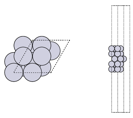
It is always a good idea to visualize the geometries to make sure they look reasonable.
import matplotlib.pyplot as plt
from ase.visualize.plot import plot_atoms

fig, axs = plt.subplots(1, 2)
plot_atoms(slab, axs[0])
plot_atoms(slab, axs[1], rotation=("-90x"))
axs[0].set_axis_off()
axs[1].set_axis_off()
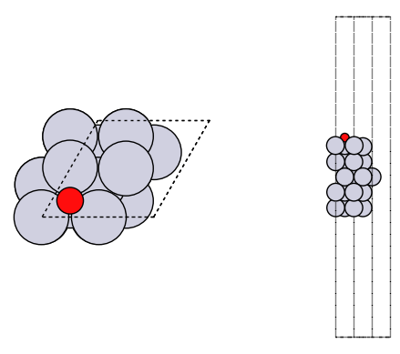
fig, axs = plt.subplots(1, 2)
plot_atoms(adslab, axs[0])
plot_atoms(adslab, axs[1], rotation=("-90x"))
axs[0].set_axis_off()
axs[1].set_axis_off()
Molecular vibrations#
from ase import Atoms
from ase.optimize import BFGS

predictor = pretrained_mlip.get_predict_unit("uma-s-1")
calc = FAIRChemCalculator(predictor, task_name="omol")

from ase.vibrations import Vibrations

n2 = Atoms("N2", [(0, 0, 0), (0, 0, 1.1)])
n2.info.update({"spin": 1, "charge": 0})
n2.calc = calc

BFGS(n2).run(fmax=0.01)
WARNING:root:device was not explicitly set, using device='cuda'.
      Step     Time          Energy          fmax
BFGS:    0 21:52:41    -2981.068009        1.645285
BFGS:    1 21:52:41    -2980.961841        6.601501
BFGS:    2 21:52:41    -2981.076753        0.203644
BFGS:    3 21:52:41    -2981.076882        0.024169
BFGS:    4 21:52:41    -2981.076883        0.000104
np.True_
vib = Vibrations(n2)
vib.run()
vib.summary()
---------------------
  #    meV     cm^-1
---------------------
  0    0.0i      0.0i
  1    0.0i      0.0i
  2    0.0       0.0
  3    2.0      16.1
  4    2.0      16.1
  5  309.2    2494.2
---------------------
Zero-point energy: 0.157 eV
Bulk alloy phase behavior#
Adapted from https://kitchingroup.cheme.cmu.edu/dft-book/dft.html#orgheadline29
We manually compute the formation energy of pure compounds and some alloy compositions to assess stability.
from ase.atoms import Atom, Atoms
from ase.filters import FrechetCellFilter
from ase.optimize import FIRE
from fairchem.core import FAIRChemCalculator, pretrained_mlip

predictor = pretrained_mlip.get_predict_unit("uma-s-1")

cu = Atoms(
    [Atom("Cu", [0.000, 0.000, 0.000])],
    cell=[[1.818, 0.000, 1.818], [1.818, 1.818, 0.000], [0.000, 1.818, 1.818]],
    pbc=True,
)
cu.calc = FAIRChemCalculator(predictor, task_name="omat")

opt = FIRE(FrechetCellFilter(cu))
opt.run(0.05, 100)

cu.get_potential_energy()
WARNING:root:device was not explicitly set, using device='cuda'.
      Step     Time          Energy          fmax
FIRE:    0 21:52:44       -3.756933        0.161999
FIRE:    1 21:52:44       -3.757594        0.110083
FIRE:    2 21:52:44       -3.758130        0.020766
-3.7581302754134702
pd = Atoms(
    [Atom("Pd", [0.000, 0.000, 0.000])],
    cell=[[1.978, 0.000, 1.978], [1.978, 1.978, 0.000], [0.000, 1.978, 1.978]],
    pbc=True,
)
pd.calc = FAIRChemCalculator(predictor, task_name="omat")

opt = FIRE(FrechetCellFilter(pd))
opt.run(0.05, 100)

pd.get_potential_energy()
      Step     Time          Energy          fmax
FIRE:    0 21:52:45       -5.211726        0.240058
FIRE:    1 21:52:45       -5.213070        0.131577
FIRE:    2 21:52:45       -5.213503        0.060260
FIRE:    3 21:52:45       -5.213528        0.051645
FIRE:    4 21:52:45       -5.213565        0.035871
-5.213564711544393
Alloy formation energies#
cupd1 = Atoms(
    [Atom("Cu", [0.000, 0.000, 0.000]), Atom("Pd", [-1.652, 0.000, 2.039])],
    cell=[[0.000, -2.039, 2.039], [0.000, 2.039, 2.039], [-3.303, 0.000, 0.000]],
    pbc=True,
)  # Note pbc=True is important, it is not the default and OMAT

cupd1.calc = FAIRChemCalculator(predictor, task_name="omat")

opt = FIRE(FrechetCellFilter(cupd1))
opt.run(0.05, 100)

cupd1.get_potential_energy()
      Step     Time          Energy          fmax
FIRE:    0 21:52:45       -9.202820        0.142029
FIRE:    1 21:52:45       -9.203042        0.127498
FIRE:    2 21:52:45       -9.203371        0.101174
FIRE: 3 21:52:45 -9.203669 0.068563
FIRE:    4 21:52:45       -9.203892        0.060712
FIRE:    5 21:52:45       -9.204129        0.078850
FIRE: 6 21:52:46 -9.204490 0.081599
FIRE:    7 21:52:46       -9.204987        0.069264
FIRE:    8 21:52:46       -9.205592        0.045645
-9.205591734189348
cupd2 = Atoms(
    [
        Atom("Cu", [-0.049, 0.049, 0.049]),
        Atom("Cu", [-11.170, 11.170, 11.170]),
        Atom("Pd", [-7.415, 7.415, 7.415]),
        Atom("Pd", [-3.804, 3.804, 3.804]),
    ],
    cell=[[-5.629, 3.701, 5.629], [-3.701, 5.629, 5.629], [-5.629, 5.629, 3.701]],
    pbc=True,
)
cupd2.calc = FAIRChemCalculator(predictor, task_name="omat")

opt = FIRE(FrechetCellFilter(cupd2))
opt.run(0.05, 100)

cupd2.get_potential_energy()
      Step     Time          Energy          fmax
FIRE:    0 21:52:46      -18.126594        0.181633
FIRE:    1 21:52:46      -18.127546        0.162952
FIRE:    2 21:52:46      -18.129065        0.127294
FIRE: 3 21:52:46 -18.130533 0.078068
FIRE: 4 21:52:46 -18.131347 0.021487
-18.13134681371561
# Delta Hf cupd-1 = -0.11 eV/atom
hf1 = (
    cupd1.get_potential_energy() - cu.get_potential_energy() - pd.get_potential_energy()
)
hf1
-0.23389674723148435
# DFT: Delta Hf cupd-2 = -0.04 eV/atom
hf2 = (
    cupd2.get_potential_energy()
    - 2 * cu.get_potential_energy()
    - 2 * pd.get_potential_energy()
)
hf2
-0.18795683979988276
hf1 - hf2, (-0.11 - -0.04)
(-0.04593990743160159, -0.07)
These indicate that cupd-1 and cupd-2 are both more stable than phase separated Cu and Pd, and that cupd-1 is more stable than cupd-2. The absolute formation energies differ from the DFT references, but the relative differences are quite close. The absolute differences could be due to DFT parameter choices (XC, psp, etc.).
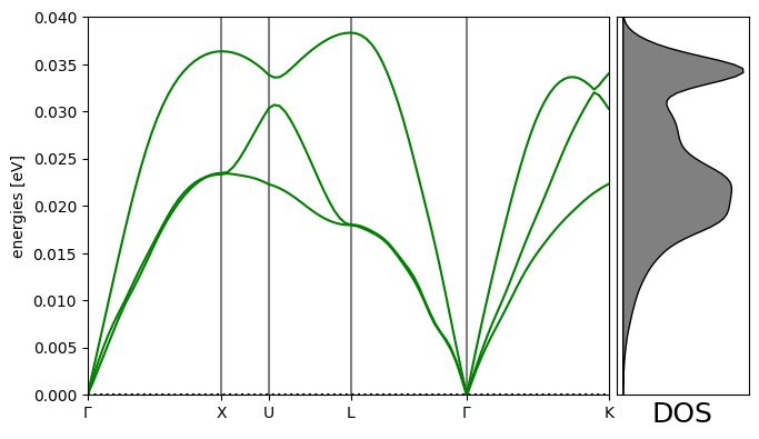
Phonon calculation#
This takes 4-10 minutes. Adapted from https://wiki.fysik.dtu.dk/ase/ase/phonons.html#example.
Phonons have applications in computing the stability and free energy of solids. See:
https://www.sciencedirect.com/science/article/pii/S1359646215003127
https://iopscience.iop.org/book/mono/978-0-7503-2572-1/chapter/bk978-0-7503-2572-1ch1
from ase.build import bulk
from ase.phonons import Phonons

predictor = pretrained_mlip.get_predict_unit("uma-s-1")
calc = FAIRChemCalculator(predictor, task_name="omat")

# Setup crystal
atoms = bulk("Al", "fcc", a=4.05)

# Phonon calculator
N = 7
ph = Phonons(atoms, calc, supercell=(N, N, N), delta=0.05)
ph.run()

# Read forces and assemble the dynamical matrix
ph.read(acoustic=True)
ph.clean()

path = atoms.cell.bandpath("GXULGK", npoints=100)
bs = ph.get_band_structure(path)

dos = ph.get_dos(kpts=(20, 20, 20)).sample_grid(npts=100, width=1e-3)
WARNING:root:device was not explicitly set, using device='cuda'.
WARNING, 1 imaginary frequencies at q = ( 0.00,  0.00,  0.00) ; (omega_q = 7.041e-09*i)
WARNING, 1 imaginary frequencies at q = ( 0.00,  0.00,  0.00) ; (omega_q = 7.041e-09*i)
# Plot the band structure and DOS:
import matplotlib.pyplot as plt  # noqa

fig = plt.figure(figsize=(7, 4))
ax = fig.add_axes([0.12, 0.07, 0.67, 0.85])

emax = 0.04
bs.plot(ax=ax, emin=0.0, emax=emax)

dosax = fig.add_axes([0.8, 0.07, 0.17, 0.85])
dosax.fill_between(
    dos.get_weights(),
    dos.get_energies(),
    y2=0,
    color="grey",
    edgecolor="k",
    lw=1,
)

dosax.set_ylim(0, emax)
dosax.set_yticks([])
dosax.set_xticks([])
dosax.set_xlabel("DOS", fontsize=18);
Transition States (NEBs)#
Nudged elastic band calculations are among the most costly calculations we do. UMA makes these quicker!
Get initial state
Get final state
Construct band and interpolate the images
Relax the band
Analyze and plot the band.
We explore diffusion of an O adatom from an hcp to an fcc site on Pt(111).
Initial state#
from ase.build import add_adsorbate, fcc111, molecule
from ase.optimize import LBFGS
from fairchem.core import FAIRChemCalculator, pretrained_mlip

predictor = pretrained_mlip.get_predict_unit("uma-s-1")
calc = FAIRChemCalculator(predictor, task_name="oc20")

# Set up your system as an ASE atoms object
initial = fcc111("Pt", (3, 3, 3), vacuum=8, periodic=True)

adsorbate = molecule("O")
add_adsorbate(initial, adsorbate, 2.0, "fcc")
initial.calc = calc

# Set up LBFGS dynamics object
opt = LBFGS(initial)
opt.run(0.05, 100)
print(initial.get_potential_energy())
WARNING:root:device was not explicitly set, using device='cuda'.
       Step     Time          Energy          fmax
LBFGS:    0 21:52:56     -141.329801        3.509944
LBFGS:    1 21:52:56     -141.719928        3.515034
LBFGS:    2 21:52:56     -142.980943        2.978368
LBFGS:    3 21:52:56     -143.684058        0.968200
LBFGS:    4 21:52:56     -143.787056        1.271672
LBFGS:    5 21:52:56     -143.858780        0.874625
LBFGS:    6 21:52:56     -143.933924        0.170912
LBFGS:    7 21:52:56     -143.937118        0.152462
LBFGS:    8 21:52:56     -143.944597        0.122234
LBFGS:    9 21:52:56     -143.948826        0.109289
LBFGS:   10 21:52:57     -143.952234        0.069971
LBFGS:   11 21:52:57     -143.953716        0.080111
LBFGS:   12 21:52:57     -143.955176        0.083489
LBFGS:   13 21:52:57     -143.956801        0.066262
LBFGS:   14 21:52:57     -143.958312        0.031495
-143.9583123027719
Final state#
# Set up your system as an ASE atoms object
final = fcc111("Pt", (3, 3, 3), vacuum=8, periodic=True)

adsorbate = molecule("O")
add_adsorbate(final, adsorbate, 2.0, "hcp")
final.calc = FAIRChemCalculator(predictor, task_name="oc20")

# Set up LBFGS dynamics object
opt = LBFGS(final)
opt.run(0.05, 100)
print(final.get_potential_energy())
       Step     Time          Energy          fmax
LBFGS:    0 21:52:57     -141.282604        3.340431
LBFGS:    1 21:52:57     -141.659793        3.323328
LBFGS:    2 21:52:57     -142.891404        2.596618
LBFGS:    3 21:52:57     -143.418901        1.225930
LBFGS:    4 21:52:57     -143.484096        0.977174
LBFGS:    5 21:52:57     -143.606344        0.136708
LBFGS:    6 21:52:57     -143.610842        0.118672
LBFGS:    7 21:52:58     -143.613319        0.100140
LBFGS:    8 21:52:58     -143.615008        0.078482
LBFGS:    9 21:52:58     -143.616454        0.051593
LBFGS:   10 21:52:58     -143.617140        0.033146
-143.61714008444915
Setup and relax the band#
from ase.mep import NEB

images = [initial]
for i in range(3):
    image = initial.copy()
    image.calc = FAIRChemCalculator(predictor, task_name="oc20")
    images.append(image)

images.append(final)


neb = NEB(images)
neb.interpolate()

opt = LBFGS(neb, trajectory="neb.traj")
opt.run(0.05, 100)
       Step     Time          Energy          fmax
LBFGS:    0 21:52:58     -143.193978        3.039289
LBFGS: 1 21:52:58 -143.360196 1.460894
LBFGS: 2 21:52:59 -143.411349 0.450309
LBFGS: 3 21:52:59 -143.423401 0.447560
LBFGS: 4 21:52:59 -143.443052 0.476377
LBFGS: 5 21:52:59 -143.459314 0.378516
LBFGS: 6 21:53:00 -143.469905 0.211698
LBFGS: 7 21:53:00 -143.474784 0.177269
LBFGS: 8 21:53:00 -143.475807 0.183701
LBFGS: 9 21:53:00 -143.477287 0.178498
LBFGS: 10 21:53:01 -143.478790 0.167185
LBFGS: 11 21:53:01 -143.479388 0.094902
LBFGS: 12 21:53:01 -143.479540 0.096952
LBFGS: 13 21:53:01 -143.479789 0.100267
LBFGS: 14 21:53:02 -143.480348 0.124768
LBFGS: 15 21:53:02 -143.481008 0.092785
LBFGS: 16 21:53:02 -143.481432 0.050531
LBFGS: 17 21:53:02 -143.481732 0.040594
np.True_
from ase.mep import NEBTools

NEBTools(neb.images).plot_band();
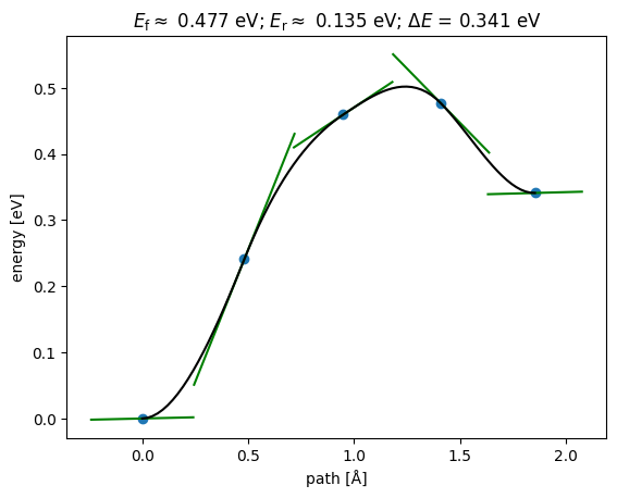
This could be a good initial guess to initialize an NEB in DFT.
Ideas for things you can do with UMA#
FineTuna - use it for initial geometry optimizations then do DFT
a. https://iopscience.iop.org/article/10.1088/2632-2153/ac8fe0
b. https://iopscience.iop.org/article/10.1088/2632-2153/ad37f0
AdsorbML - prescreen adsorption sites to find relevant ones
a. https://www.nature.com/articles/s41524-023-01121-5
CatTsunami - screen NEBs more thoroughly
a. https://pubs.acs.org/doi/10.1021/acscatal.4c04272
Free energy estimations - compute vibrational modes and use them to estimate vibrational entropy
a. https://pubs.acs.org/doi/10.1021/acs.jpcc.4c07477
Massive screening of catalyst surface properties (685M relaxations)
a. https://arxiv.org/abs/2411.11783
Advanced applications#
These take a while to run.
AdsorbML#
It is so cheap to run these calculations that we can screen a broad range of adsorbate sites and rank them in stability. The AdsorbML approach automates this. This takes quite a while to run here, and we don’t do it in the workshop.
Expert adsorption energies#
This tutorial reproduces Fig 6b from the following paper: Zhou, Jing, et al. “Enhanced Catalytic Activity of Bimetallic Ordered Catalysts for Nitrogen Reduction Reaction by Perturbation of Scaling Relations.” ACS Catalysis 134 (2023): 2190-2201 (https://doi.org/10.1021/acscatal.2c05877).
This takes up to an hour with a GPU, and much longer with a CPU.
CatTsunami#
The CatTsunami tutorial is an example of enumerating initial and final states, and computing reaction paths between them with UMA.
Acknowledgements#
This tutorial was originally compiled by John Kitchin (CMU) for the NAM29 catalysis tutorial session, using a variety of resources from the FAIR chemistry repository.