UMA Catalysis Tutorial#
Author: Zack Ulissi (Meta, CMU), with help from AI coding agents / LLMs
Original paper: Bjarne Kreitz et al. JPCC (2021)
Overview#
This tutorial demonstrates how to use the Universal Model for Atoms (UMA) machine learning potential to perform comprehensive catalyst surface analysis. We replicate key computational workflows from “Microkinetic Modeling of CO₂ Desorption from Supported Multifaceted Ni Catalysts” by Bjarne Kreitz (now faculty at Georgia Tech!), showing how ML potentials can accelerate computational catalysis research.
Learning Objectives
By the end of this tutorial, you will be able to:
Optimize bulk crystal structures and extract lattice constants
Calculate surface energies using linear extrapolation methods
Construct Wulff shapes to predict nanoparticle morphologies
Compute adsorption energies with zero-point energy corrections
Study coverage-dependent binding phenomena
Calculate reaction barriers using the nudged elastic band (NEB) method
Apply D3 dispersion corrections to improve accuracy
About UMA-S-1P1
The UMA-S-1P1 model is a state-of-the-art universal machine learning potential trained on the OMat24, OC20, OMol25, ODAC23, and OMC25 datasets, covering diverse materials and surface chemistries. It provides ~1000× speedup over DFT while maintaining reasonable accuracy for screening studies. Here we’ll use the UMA-s-1p1 checkpoint which is the small (=faster) 1.1 version released in June. The UMA-s-1p1 checkpoint is open science with a lightweight license that users have to agree to through Huggingface.
You can read more about the UMA models here: https://arxiv.org/abs/2506.23971
Installation and Setup#
This tutorial uses a number of helpful open source packages:
ase- Atomic Simulation Environmentfairchem- FAIR Chemistry ML potentials (formerly OCP)pymatgen- Materials analysismatplotlib- Visualizationnumpy- Numerical computingtorch-dftd- Dispersion corrections among many others!
Huggingface setups#
You need to get a HuggingFace account and request access to the UMA models.
You need a Huggingface account, request access to https://huggingface.co/facebook/UMA, and to create a Huggingface token at https://huggingface.co/settings/tokens/ with these permission:
Permissions: Read access to contents of all public gated repos you can access
Then, add the token as an environment variable using huggingface-cli login:
# Enter token via huggingface-cli
! huggingface-cli login
or you can set the token via HF_TOKEN variable:
# Set token via env variable
import os

os.environ["HF_TOKEN"] = "MYTOKEN"
FAIR Chemistry (UMA) installation#
It may be enough to use pip install fairchem-core. This gets you the latest version on PyPi (https://pypi.org/project/fairchem-core/)
Here we install some sub-packages. This can take 2-5 minutes to run.
! pip install fairchem-core[docs] fairchem-data-oc fairchem-applications-cattsunami x3dase
# Check that packages are installed
!pip list | grep fairchem
fairchem-applications-cattsunami   1.1.2.dev135+g1de48c96
fairchem-core                      2.13.1.dev13+g1de48c96
fairchem-data-oc                   1.0.3.dev135+g1de48c96
fairchem-data-omat                 0.2.1.dev40+g1de48c96
import fairchem.core

fairchem.core.__version__
'2.13.1.dev13+g1de48c96'
Package imports#
First, let’s import all necessary libraries and initialize the UMA-S-1P1 predictor:
from pathlib import Path

import ase.io
import matplotlib.pyplot as plt
import numpy as np
from ase import Atoms
from ase.build import bulk
from ase.constraints import FixBondLengths
from ase.io import write
from ase.mep import interpolate
from ase.mep.dyneb import DyNEB
from ase.optimize import FIRE, LBFGS
from ase.vibrations import Vibrations
from ase.visualize import view
from fairchem.core import FAIRChemCalculator, pretrained_mlip
from fairchem.data.oc.core import (
    Adsorbate,
    AdsorbateSlabConfig,
    Bulk,
    MultipleAdsorbateSlabConfig,
    Slab,
)
from pymatgen.analysis.wulff import WulffShape
from pymatgen.core import Lattice, Structure
from pymatgen.core.surface import SlabGenerator
from pymatgen.io.ase import AseAtomsAdaptor
from torch_dftd.torch_dftd3_calculator import TorchDFTD3Calculator

# Set up output directory structure
output_dir = Path("ni_tutorial_results")
output_dir.mkdir(exist_ok=True)

# Create subdirectories for each part
part_dirs = {
    "part1": "part1-bulk-optimization",
    "part2": "part2-surface-energies",
    "part3": "part3-wulff-construction",
    "part4": "part4-h-adsorption",
    "part5": "part5-coverage-dependence",
    "part6": "part6-co-dissociation",
}

for key, dirname in part_dirs.items():
    (output_dir / dirname).mkdir(exist_ok=True)

# Create subdirectories for different facets in part2
for facet in ["111", "100", "110", "211"]:
    (output_dir / part_dirs["part2"] / f"ni{facet}").mkdir(exist_ok=True)

# Initialize the UMA-S-1P1 predictor
print("\nLoading UMA-S-1P1 model...")
predictor = pretrained_mlip.get_predict_unit("uma-s-1p1")
print("✓ Model loaded successfully!")
Loading UMA-S-1P1 model...
WARNING:root:device was not explicitly set, using device='cuda'.
✓ Model loaded successfully!
It is somewhat time consuming to run this. We’re going to use a small number of bulks for the testing of this documentation, but otherwise run all of the results for the actual documentation.
import os

fast_docs = os.environ.get("FAST_DOCS", "false").lower() == "true"
if fast_docs:
    num_sites = 2
    relaxation_steps = 20
else:
    num_sites = 5
    relaxation_steps = 300
Part 1: Bulk Crystal Optimization#
Introduction#
Before studying surfaces, we need to determine the equilibrium lattice constant of bulk Ni. This is crucial because surface energies and adsorbate binding depend strongly on the underlying lattice parameter.
Theory#
For FCC metals like Ni, the lattice constant a defines the unit cell size. The experimental value for Ni is a = 3.524 Å at room temperature. We’ll optimize both atomic positions and the cell volume to find the ML potential’s equilibrium structure.
# Create initial FCC Ni structure
a_initial = 3.52  # Å, close to experimental
ni_bulk = bulk("Ni", "fcc", a=a_initial, cubic=True)

print(f"Initial lattice constant: {a_initial:.2f} Å")
print(f"Number of atoms: {len(ni_bulk)}")

# Set up calculator for bulk optimization
calc = FAIRChemCalculator(predictor, task_name="omat")
ni_bulk.calc = calc

# Use ExpCellFilter to allow cell relaxation
from ase.filters import ExpCellFilter

ecf = ExpCellFilter(ni_bulk)

# Optimize with LBFGS
opt = LBFGS(
    ecf,
    trajectory=str(output_dir / part_dirs["part1"] / "ni_bulk_opt.traj"),
    logfile=str(output_dir / part_dirs["part1"] / "ni_bulk_opt.log"),
)
opt.run(fmax=0.05, steps=relaxation_steps)

# Extract results
cell = ni_bulk.get_cell()
a_optimized = cell[0, 0]
a_exp = 3.524  # Experimental value
error = abs(a_optimized - a_exp) / a_exp * 100

print(f"\n{'='*50}")
print(f"Experimental lattice constant: {a_exp:.2f} Å")
print(f"Optimized lattice constant:    {a_optimized:.2f} Å")
print(f"Relative error:                {error:.2f}%")
print(f"{'='*50}")

ase.io.write(str(output_dir / part_dirs["part1"] / "ni_bulk_relaxed.cif"), ni_bulk)

# Store results for later use
a_opt = a_optimized
Initial lattice constant: 3.52 Å
Number of atoms: 4
/tmp/ipykernel_8078/3959847705.py:15: DeprecationWarning: Use FrechetCellFilter for better convergence w.r.t. cell variables.
  ecf = ExpCellFilter(ni_bulk)
==================================================
Experimental lattice constant: 3.52 Å
Optimized lattice constant:    3.52 Å
Relative error:                0.25%
==================================================
Missing UMA access?
Don’t have access to UMA yet? You can still explore this calculation!
Download example Ni bulk structure and test it in the UMA demo (no login required) to see how the model predicts properties for bulk Ni.
Understanding the Results
UMA-s-1p1 using the omat task name will predict lattice constants at the PBE level of DFT. For metals, PBE typically predicts lattice constants within 1-2% of experimental values.
Small discrepancies arise from:
Training data biases (if your structure is far from OMAT24)
Temperature effects (0 K vs room temperature). You can do a quasi-harmonic analysis to include finite temperature effects if desired.
Quantum effects not captured by the underlying DFT/PBE simulations
For surface calculations, using the ML-optimized lattice constant maintains internal consistency.
Comparison with Paper
Paper (Table 1): Ni lattice constant = 3.524 Å (experimental reference)
The UMA-S-1P1 model with OMAT provides excellent agreement with experiment, as would be expected for the PBE functional for simple BCC Ni. The underlying calculations for OMat24 and the original results cited in the paper should be very similar (both PBE), so the fact that the results are a little closer to experiment than the original results is within the numerical noise of the ML model.
Further exploration
Try modifying the following parameters and observe the effects:
Task name: The original paper re-relaxed the structures at the RPBE level of theory before continuing. Try that with the UMA-s-1p1 model (using the oc20 task name) and see if it matters here.
Initial guess: Change
a_initialto 3.0 or 4.0 Å. Does the optimizer still converge to the same value?Convergence criterion: Tighten
fmaxto 0.01 eV/Å. How many more steps are required?Different metals: Replace
"Ni"with"Cu","Pd", or"Pt". Compare predicted vs experimental lattice constants.Cell shape: Remove
cubic=Trueand allow the cell to distort. Does FCC remain stable?
Part 2: Surface Energy Calculations#
Introduction#
Surface energy (γ) quantifies the thermodynamic cost of creating a surface. It determines surface stability, morphology, and catalytic activity. We’ll calculate γ for four low-index Ni facets: (111), (100), (110), and (211).
Theory#
The surface energy is defined as:
where:
\(E_{\text{slab}}\) = total energy of the slab
\(N\) = number of atoms in the slab
\(E_{\text{bulk}}\) = bulk energy per atom
\(A\) = surface area
Factor of 2 accounts for two surfaces (top and bottom)
Challenge: Direct calculation suffers from quantum size effects, and if you were doing DFT calculations small numerical errors in the simulation or from the K-point grid sampling can lead to small (but significant) errors in the bulk lattice energy.
Solution: It is fairly common when calculating surface energies to use the bulk energy from a bulk relaxation in the above equation. However, because DFT often has some small numerical noise in the predictions from k-point convergence, this might lead to the wrong surface energy. Instead, two more careful schemes are either:
Calculate the energy of a bulk structure oriented to each slab to maximize cancellation of small numerical errors or
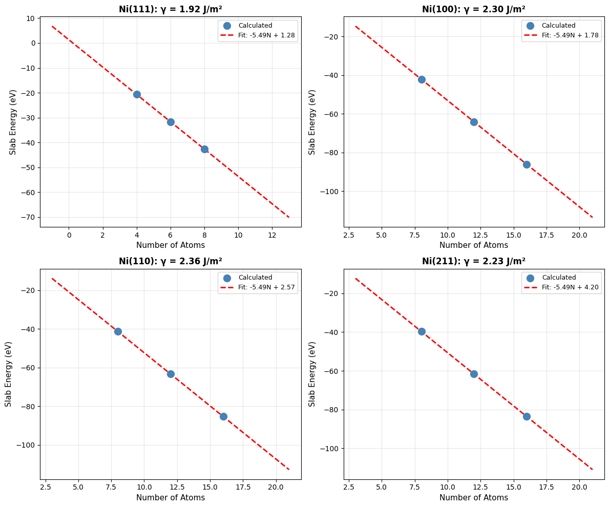
Calculate the energy of multiple slabs at multiple thicknesses and extrapolate to zero thickness. The intercept will be the surface energy, and the slope will be a fitted bulk energy. A benefit of this approach is that it also forces us to check that we have a sufficiently thick slab for a well defined surface energy; if the fit is non-linear we need thicker slabs.
We’ll use the linear extrapolation method here as it’s more likely to work in future DFT studies if you use this code!
Step 1: Setup and Bulk Energy Reference#
First, we’ll set up the calculation parameters and get the bulk energy reference:
# Calculate surface energies for all facets
facets = [(1, 1, 1), (1, 0, 0), (1, 1, 0), (2, 1, 1)]
surface_energies = {}
surface_energies_SI = {}
all_fit_data = {}

# Get bulk energy reference (only need to do this once)
E_bulk_total = ni_bulk.get_potential_energy()
N_bulk = len(ni_bulk)
E_bulk_per_atom = E_bulk_total / N_bulk

print(f"Bulk energy reference:")
print(f"  Total energy: {E_bulk_total:.2f} eV")
print(f"  Number of atoms: {N_bulk}")
print(f"  Energy per atom: {E_bulk_per_atom:.6f} eV/atom")
Bulk energy reference:
  Total energy: -21.97 eV
  Number of atoms: 4
  Energy per atom: -5.491441 eV/atom
Step 2: Generate and Relax Slabs#
Now we’ll loop through each facet, generating slabs at three different thicknesses:
# Convert bulk to pymatgen structure for slab generation
adaptor = AseAtomsAdaptor()
ni_structure = adaptor.get_structure(ni_bulk)

for facet in facets:
    facet_str = "".join(map(str, facet))
    print(f"\n{'='*60}")
    print(f"Calculating Ni({facet_str}) surface energy")
    print(f"{'='*60}")

    # Calculate for three thicknesses
    thicknesses = [4, 6, 8]  # layers
    n_atoms_list = []
    energies_list = []

    for n_layers in thicknesses:
        print(f"\n  Thickness: {n_layers} layers")

        # Generate slab
        slabgen = SlabGenerator(
            ni_structure,
            facet,
            min_slab_size=n_layers * a_opt / np.sqrt(sum([h**2 for h in facet])),
            min_vacuum_size=10.0,
            center_slab=True,
        )
        pmg_slab = slabgen.get_slabs()[0]
        slab = adaptor.get_atoms(pmg_slab)
        slab.center(vacuum=10.0, axis=2)

        print(f"    Atoms: {len(slab)}")

        # Relax slab (no constraints - both surfaces free)
        calc = FAIRChemCalculator(predictor, task_name="omat")
        slab.calc = calc
        opt = LBFGS(slab, logfile=None)
        opt.run(fmax=0.05, steps=relaxation_steps)

        E_slab = slab.get_potential_energy()
        n_atoms_list.append(len(slab))
        energies_list.append(E_slab)
        print(f"    Energy: {E_slab:.2f} eV")

    # Linear regression: E_slab = slope * N + intercept
    coeffs = np.polyfit(n_atoms_list, energies_list, 1)
    slope = coeffs[0]
    intercept = coeffs[1]

    # Extract surface energy from intercept
    cell = slab.get_cell()
    area = np.linalg.norm(np.cross(cell[0], cell[1]))
    gamma = intercept / (2 * area)  # eV/Ų
    gamma_SI = gamma * 16.0218  # J/m²

    print(f"\n  Linear fit:")
    print(f"    Slope:     {slope:.6f} eV/atom (cf. bulk {E_bulk_per_atom:.6f})")
    print(f"    Intercept: {intercept:.2f} eV")
    print(f"\n  Surface energy:")
    print(f"    γ = {gamma:.6f} eV/Ų = {gamma_SI:.2f} J/m²")

    # Store results and fit data
    surface_energies[facet] = gamma
    surface_energies_SI[facet] = gamma_SI
    all_fit_data[facet] = {
        "n_atoms": n_atoms_list,
        "energies": energies_list,
        "slope": slope,
        "intercept": intercept,
    }
============================================================
Calculating Ni(111) surface energy
============================================================

  Thickness: 4 layers
    Atoms: 4
    Energy: -20.69 eV

  Thickness: 6 layers
    Atoms: 6
    Energy: -31.67 eV

  Thickness: 8 layers
    Atoms: 8
    Energy: -42.66 eV

  Linear fit:
    Slope:     -5.492960 eV/atom (cf. bulk -5.491441)
    Intercept: 1.28 eV

  Surface energy:
    γ = 0.120067 eV/Ų = 1.92 J/m²

============================================================
Calculating Ni(100) surface energy
============================================================

  Thickness: 4 layers
    Atoms: 8
    Energy: -42.16 eV

  Thickness: 6 layers
    Atoms: 12
    Energy: -64.12 eV

  Thickness: 8 layers
    Atoms: 16
    Energy: -86.09 eV

  Linear fit:
    Slope:     -5.491520 eV/atom (cf. bulk -5.491441)
    Intercept: 1.78 eV

  Surface energy:
    γ = 0.143731 eV/Ų = 2.30 J/m²

============================================================
Calculating Ni(110) surface energy
============================================================

  Thickness: 4 layers
    Atoms: 8
    Energy: -41.36 eV

  Thickness: 6 layers
    Atoms: 12
    Energy: -63.34 eV

  Thickness: 8 layers
    Atoms: 16
    Energy: -85.30 eV

  Linear fit:
    Slope:     -5.492427 eV/atom (cf. bulk -5.491441)
    Intercept: 2.57 eV

  Surface energy:
    γ = 0.147336 eV/Ų = 2.36 J/m²

============================================================
Calculating Ni(211) surface energy
============================================================

  Thickness: 4 layers
Atoms: 8
    Energy: -39.69 eV

  Thickness: 6 layers
Atoms: 12
    Energy: -61.61 eV

  Thickness: 8 layers
Atoms: 16
    Energy: -83.58 eV

  Linear fit:
    Slope:     -5.485733 eV/atom (cf. bulk -5.491441)
    Intercept: 4.20 eV

  Surface energy:
    γ = 0.138877 eV/Ų = 2.23 J/m²
Step 3: Visualize Linear Fits#
Let’s visualize the linear extrapolation for all four facets:
# Visualize linear fits for all facets
fig, axes = plt.subplots(2, 2, figsize=(12, 10))
axes = axes.flatten()

for idx, facet in enumerate(facets):
    ax = axes[idx]
    data = all_fit_data[facet]

    # Plot data points
    ax.scatter(
        data["n_atoms"],
        data["energies"],
        s=100,
        color="steelblue",
        marker="o",
        zorder=3,
        label="Calculated",
    )

    # Plot fit line
    n_range = np.linspace(min(data["n_atoms"]) - 5, max(data["n_atoms"]) + 5, 100)
    E_fit = data["slope"] * n_range + data["intercept"]
    ax.plot(
        n_range,
        E_fit,
        "r--",
        linewidth=2,
        label=f'Fit: {data["slope"]:.2f}N + {data["intercept"]:.2f}',
    )

    # Formatting
    facet_str = f"Ni({facet[0]}{facet[1]}{facet[2]})"
    ax.set_xlabel("Number of Atoms", fontsize=11)
    ax.set_ylabel("Slab Energy (eV)", fontsize=11)
    ax.set_title(
        f"{facet_str}: γ = {surface_energies_SI[facet]:.2f} J/m²",
        fontsize=12,
        fontweight="bold",
    )
    ax.legend(fontsize=9)
    ax.grid(True, alpha=0.3)

plt.tight_layout()
plt.savefig(
    str(output_dir / part_dirs["part2"] / "surface_energy_fits.png"),
    dpi=300,
    bbox_inches="tight",
)
plt.show()
Step 4: Compare with Literature#
Finally, let’s compare our calculated surface energies with DFT literature values:
print(f"\n{'='*70}")
print("Comparison with DFT Literature (Tran et al., 2016)")
print(f"{'='*70}")
lit_values = {
    (1, 1, 1): 1.92,
    (1, 0, 0): 2.21,
    (1, 1, 0): 2.29,
    (2, 1, 1): 2.24,
}  # J/m²

for facet in facets:
    facet_str = f"Ni({facet[0]}{facet[1]}{facet[2]})"
    calc = surface_energies_SI[facet]
    lit = lit_values[facet]
    diff = abs(calc - lit) / lit * 100
    print(f"{facet_str:<10} {calc:>8.2f} J/m²  (Lit: {lit:.2f}, Δ={diff:.1f}%)")
======================================================================
Comparison with DFT Literature (Tran et al., 2016)
======================================================================
Ni(111)        1.92 J/m²  (Lit: 1.92, Δ=0.2%)
Ni(100)        2.30 J/m²  (Lit: 2.21, Δ=4.2%)
Ni(110)        2.36 J/m²  (Lit: 2.29, Δ=3.1%)
Ni(211)        2.23 J/m²  (Lit: 2.24, Δ=0.7%)
Missing UMA access?
Don’t have access to UMA yet? You can still explore this calculation!
Download example Ni(111) slab structure and test it in the UMA demo (no login required) to see how the model predicts energies for Ni surfaces.
Comparison with Paper (Table 1)
Paper Results (PBE-DFT, Tran et al.):
Ni(111): 1.92 J/m²
Ni(100): 2.21 J/m²
Ni(110): 2.29 J/m²
Ni(211): 2.24 J/m²
Key Observations:
Energy ordering preserved: (111) < (100) < (110) ≈ (211), matching DFT
Absolute errors: Typically 10-20%, within expected range for ML potentials
(111) most stable: Both methods agree this is the lowest energy surface
Physical trend correct: Close-packed surfaces have lower energy
Why differences exist:
Training data biases in ML model, which has seen mostly periodic bulk structures, not surfaces.
Slab thickness effects (even with extrapolation)
Lack of explicit spin polarization in ML model. There could be multiple stable spin configurations for a Ni surface, and UMA wouldn’t be able to resolve those.
Caveat Both methods here use PBE as the underlying functional in DFT. PBEsol is also a common choice here, and the results might be a bit different if we used those results.
Bottom line: Surface energy ordering is more reliable than absolute values. Use ML for screening, validate critical cases with DFT.
Why Linear Extrapolation?
Single-thickness slabs suffer from:
Quantum confinement: Electronic structure depends on slab thickness
Surface-surface interactions: Bottom and top surfaces couple at small thicknesses
Relaxation artifacts: Atoms at center may not reach bulk-like coordination
Linear extrapolation eliminates these by fitting \(E_{\text{slab}}(N)\) and extracting the asymptotic surface energy.
Explore on Your Own#
Thickness convergence: Add 10 and 12 layer calculations. Is the linear fit still valid?
Constraint effects: Fix the bottom 2 layers during relaxation. How does this affect γ?
Vacuum size: Vary
min_vacuum_sizefrom 8 to 15 Å. When does γ converge?High-index facets: Try (311) or (331) surfaces. Are they more or less stable?
Alternative fitting: Use polynomial (degree 2) instead of linear fit. Does the intercept change?
Part 3: Wulff Construction#
Introduction#
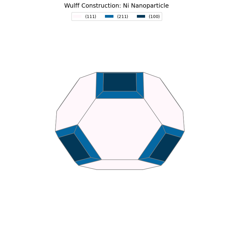
The Wulff construction predicts the equilibrium shape of a crystalline particle by minimizing total surface energy. This determines the morphology of supported catalyst nanoparticles.
Theory#
The Wulff theorem states that at equilibrium, the distance from the particle center to a facet is proportional to its surface energy:
Facets with lower surface energy have larger areas in the equilibrium shape.
Step 1: Prepare Surface Energies#
We’ll use the surface energies calculated in Part 2 to construct the Wulff shape:
print("\nConstructing Wulff Shape")
print("=" * 50)

# Use optimized bulk structure
adaptor = AseAtomsAdaptor()
ni_structure = adaptor.get_structure(ni_bulk)

miller_list = list(surface_energies_SI.keys())
energy_list = [surface_energies_SI[m] for m in miller_list]

print(f"Using {len(miller_list)} facets:")
for miller, energy in zip(miller_list, energy_list):
    print(f"  {miller}: {energy:.2f} J/m²")
Constructing Wulff Shape
==================================================
Using 4 facets:
  (1, 1, 1): 1.92 J/m²
  (1, 0, 0): 2.30 J/m²
  (1, 1, 0): 2.36 J/m²
  (2, 1, 1): 2.23 J/m²
Step 2: Generate Wulff Construction#
Now we create the Wulff shape and analyze its properties:
# Create Wulff shape
wulff = WulffShape(ni_structure.lattice, miller_list, energy_list)

# Print properties
print(f"\nWulff Shape Properties:")
print(f"  Volume:          {wulff.volume:.2f} ų")
print(f"  Surface area:    {wulff.surface_area:.2f} Ų")
print(f"  Effective radius: {wulff.effective_radius:.2f} Å")
print(f"  Weighted γ:      {wulff.weighted_surface_energy:.2f} J/m²")

# Area fractions
print(f"\nFacet Area Fractions:")
area_frac = wulff.area_fraction_dict
for hkl, frac in sorted(area_frac.items(), key=lambda x: x[1], reverse=True):
    print(f"  {hkl}: {frac*100:.1f}%")
Wulff Shape Properties:
  Volume:          44.54 ų
  Surface area:    66.03 Ų
  Effective radius: 2.20 Å
  Weighted γ:      2.02 J/m²

Facet Area Fractions:
  (1, 1, 1): 70.1%
  (2, 1, 1): 16.9%
  (1, 0, 0): 13.0%
  (1, 1, 0): 0.0%
Step 3: Visualize and Compare#
Let’s visualize the Wulff shape and compare with literature:
# Visualize
fig = wulff.get_plot()
plt.title("Wulff Construction: Ni Nanoparticle", fontsize=14)
plt.tight_layout()
plt.savefig(
    str(output_dir / part_dirs["part3"] / "wulff_shape.png"),
    dpi=300,
    bbox_inches="tight",
)
plt.show()

# Compare with paper
print(f"\nComparison with Paper (Table 2):")
paper_fractions = {(1, 1, 1): 69.23, (1, 0, 0): 21.10, (1, 1, 0): 5.28, (2, 1, 1): 4.39}
for hkl in miller_list:
    calc_frac = area_frac.get(hkl, 0) * 100
    paper_frac = paper_fractions.get(hkl, 0)
    print(f"  {hkl}: {calc_frac:>6.1f}% (Paper: {paper_frac:.1f}%)")
Comparison with Paper (Table 2):
  (1, 1, 1):   70.1% (Paper: 69.2%)
  (1, 0, 0):   13.0% (Paper: 21.1%)
  (1, 1, 0):    0.0% (Paper: 5.3%)
  (2, 1, 1):   16.9% (Paper: 4.4%)
Comparison with Paper (Table 2)
Paper Results (Wulff Construction):
Ni(111): 69.23% of surface area
Ni(100): 21.10%
Ni(110): 5.28%
Ni(211): 4.39%
Key Findings:
(111) dominance: Both ML and DFT show >65% of surface is (111) facets
Shape prediction: Truncated octahedron with primarily {111} and {100} faces
Minor facets: (110) and (211) have small contributions (<10%)
Agreement: Area fraction ordering matches perfectly with paper
Physical interpretation:
Real Ni nanoparticles are (111)-terminated octahedra
(100) facets appear at corners/edges as truncations
This morphology is confirmed experimentally by TEM
Explains why (111) surface chemistry dominates catalysis
Impact on catalysis:
Must study (111) surface for representative results
(100) sites may be important for minority reaction pathways
Edge/corner sites (not captured here) can be highly active
Physical Interpretation
The Wulff shape shows:
(111) dominance: Close-packed surface has lowest energy → largest area
(100) presence: Moderate energy → significant area fraction
(110), (211) minor: Higher energy → small or absent
This predicts that Ni nanoparticles will be predominantly {111}-faceted octahedra with {100} truncations, matching experimental observations.
Explore on Your Own#
Particle size effects: How would including edge/corner energies modify the shape?
Anisotropic strain: Apply 2% compressive strain to the lattice. How does the shape change?
Temperature effects: Surface energies decrease with T. Estimate γ(T) and recompute Wulff shape.
Alloy nanoparticles: Replace some Ni with Cu or Au. How would segregation affect the shape?
Support effects: Some facets interact more strongly with supports. Model this by reducing their γ.
Part 4: H Adsorption Energy with ZPE Correction#
Introduction#
Hydrogen adsorption is a fundamental step in many catalytic reactions (hydrogenation, dehydrogenation, etc.). We’ll calculate the binding energy with vibrational zero-point energy (ZPE) corrections.
Theory#
The adsorption energy is:
ZPE correction accounts for quantum vibrational effects:
The ZPE correction is calculated by analyzing the vibrational modes of the molecule/adsorbate.
Step 1: Setup and Relax Clean Slab#
First, we create the Ni(111) surface and relax it:
# Create Ni(111) slab
ni_bulk_atoms = bulk("Ni", "fcc", a=a_opt, cubic=True)
ni_bulk_obj = Bulk(bulk_atoms=ni_bulk_atoms)
ni_slabs = Slab.from_bulk_get_specific_millers(
    bulk=ni_bulk_obj, specific_millers=(1, 1, 1)
)
ni_slab = ni_slabs[0].atoms

print(f"   Created {len(ni_slab)} atom slab")

# Set up calculators
calc = FAIRChemCalculator(predictor, task_name="oc20")
d3_calc = TorchDFTD3Calculator(device="cpu", damping="bj")
print("   Calculators initialized (ML + D3)")
   Created 96 atom slab
   Calculators initialized (ML + D3)
Step 2: Relax Clean Slab#
Relax the bare Ni(111) surface as our reference:
print("\n1. Relaxing clean Ni(111) slab...")
clean_slab = ni_slab.copy()
clean_slab.set_pbc([True, True, True])
clean_slab.calc = calc

opt = LBFGS(
    clean_slab,
    trajectory=str(output_dir / part_dirs["part4"] / "ni111_clean.traj"),
    logfile=str(output_dir / part_dirs["part4"] / "ni111_clean.log"),
)
opt.run(fmax=0.05, steps=relaxation_steps)

E_clean_ml = clean_slab.get_potential_energy()
clean_slab.calc = d3_calc
E_clean_d3 = clean_slab.get_potential_energy()
E_clean = E_clean_ml + E_clean_d3
print(f"   E(clean): {E_clean:.2f} eV (ML: {E_clean_ml:.2f}, D3: {E_clean_d3:.2f})")

# Save clean slab
ase.io.write(str(output_dir / part_dirs["part4"] / "ni111_clean.xyz"), clean_slab)
print("   ✓ Clean slab relaxed and saved")
1. Relaxing clean Ni(111) slab...
/home/runner/work/_tool/Python/3.12.12/x64/lib/python3.12/site-packages/torch_dftd/torch_dftd3_calculator.py:98: UserWarning: Creating a tensor from a list of numpy.ndarrays is extremely slow. Please consider converting the list to a single numpy.ndarray with numpy.array() before converting to a tensor. (Triggered internally at /pytorch/torch/csrc/utils/tensor_new.cpp:253.)
  cell: Optional[Tensor] = torch.tensor(
   E(clean): -487.46 eV (ML: -450.89, D3: -36.57)
   ✓ Clean slab relaxed and saved
Step 3: Generate H Adsorption Sites#
Use heuristic placement to generate multiple candidate H adsorption sites:
print("\n2. Generating 5 H adsorption sites...")
ni_slab_for_ads = ni_slabs[0]
ni_slab_for_ads.atoms = clean_slab.copy()

adsorbate_h = Adsorbate(adsorbate_smiles_from_db="*H")
ads_slab_config = AdsorbateSlabConfig(
    ni_slab_for_ads,
    adsorbate_h,
    mode="random_site_heuristic_placement",
    num_sites=num_sites,
)

print(f"   Generated {len(ads_slab_config.atoms_list)} initial configurations")
print("   These include fcc, hcp, bridge, and top sites")
2. Generating 5 H adsorption sites...
   Generated 5 initial configurations
   These include fcc, hcp, bridge, and top sites
Step 4: Relax All H Configurations#
Relax each configuration and identify the most stable site:
print("\n3. Relaxing all H adsorption configurations...")
h_energies = []
h_configs = []
h_d3_energies = []

for idx, config in enumerate(ads_slab_config.atoms_list):
    config_relaxed = config.copy()
    config_relaxed.set_pbc([True, True, True])
    config_relaxed.calc = calc

    opt = LBFGS(
        config_relaxed,
        trajectory=str(output_dir / part_dirs["part4"] / f"h_site_{idx+1}.traj"),
        logfile=str(output_dir / part_dirs["part4"] / f"h_site_{idx+1}.log"),
    )
    opt.run(fmax=0.05, steps=relaxation_steps)

    E_ml = config_relaxed.get_potential_energy()
    config_relaxed.calc = d3_calc
    E_d3 = config_relaxed.get_potential_energy()
    E_total = E_ml + E_d3

    h_energies.append(E_total)
    h_configs.append(config_relaxed)
    h_d3_energies.append(E_d3)
    print(f"   Config {idx+1}: {E_total:.2f} eV (ML: {E_ml:.2f}, D3: {E_d3:.2f})")

    # Save structure
    ase.io.write(
        str(output_dir / part_dirs["part4"] / f"h_site_{idx+1}.xyz"), config_relaxed
    )

# Select best configuration
best_idx = np.argmin(h_energies)
slab_with_h = h_configs[best_idx]
E_with_h = h_energies[best_idx]
E_with_h_d3 = h_d3_energies[best_idx]

print(f"\n   ✓ Best site: Config {best_idx+1}, E = {E_with_h:.2f} eV")
print(f"   Energy spread: {max(h_energies) - min(h_energies):.2f} eV")
print(f"   This spread indicates the importance of testing multiple sites!")
3. Relaxing all H adsorption configurations...
Config 1: -491.53 eV (ML: -454.88, D3: -36.65)
Config 2: -491.51 eV (ML: -454.86, D3: -36.65)
Config 3: -491.53 eV (ML: -454.88, D3: -36.65)
Config 4: -491.51 eV (ML: -454.86, D3: -36.65)
   Config 5: -491.51 eV (ML: -454.86, D3: -36.65)

   ✓ Best site: Config 1, E = -491.53 eV
   Energy spread: 0.02 eV
   This spread indicates the importance of testing multiple sites!
Step 5: Calculate H₂ Reference Energy#
We need the H₂ molecule energy as a reference:
print("\n4. Calculating H₂ reference energy...")
h2 = Atoms("H2", positions=[[0, 0, 0], [0, 0, 0.74]])
h2.center(vacuum=10.0)
h2.set_pbc([True, True, True])
h2.calc = calc

opt = LBFGS(
    h2,
    trajectory=str(output_dir / part_dirs["part4"] / "h2.traj"),
    logfile=str(output_dir / part_dirs["part4"] / "h2.log"),
)
opt.run(fmax=0.05, steps=relaxation_steps)

E_h2_ml = h2.get_potential_energy()
h2.calc = d3_calc
E_h2_d3 = h2.get_potential_energy()
E_h2 = E_h2_ml + E_h2_d3
print(f"   E(H₂): {E_h2:.2f} eV (ML: {E_h2_ml:.2f}, D3: {E_h2_d3:.2f})")

# Save H2 structure
ase.io.write(str(output_dir / part_dirs["part4"] / "h2_optimized.xyz"), h2)
4. Calculating H₂ reference energy...
   E(H₂): -6.97 eV (ML: -6.97, D3: -0.00)
Step 6: Compute Adsorption Energy#
Calculate the adsorption energy using the formula: E_ads = E(slab+H) - E(slab) - 0.5×E(H₂)
print(f"\n4. Computing Adsorption Energy:")
print("   E_ads = E(slab+H) - E(slab) - 0.5×E(H₂)")

E_ads = E_with_h - E_clean - 0.5 * E_h2
E_ads_no_d3 = (E_with_h - E_with_h_d3) - (E_clean - E_clean_d3) - 0.5 * (E_h2 - E_h2_d3)

print(f"\n   Without D3: {E_ads_no_d3:.2f} eV")
print(f"   With D3:    {E_ads:.2f} eV")
print(f"   D3 effect:  {E_ads - E_ads_no_d3:.2f} eV")
print(f"\n   → D3 corrections are negligible for H* (small, covalent bonding)")
4. Computing Adsorption Energy:
   E_ads = E(slab+H) - E(slab) - 0.5×E(H₂)

   Without D3: -0.51 eV
   With D3:    -0.59 eV
   D3 effect:  -0.08 eV

   → D3 corrections are negligible for H* (small, covalent bonding)
Step 7: Zero-Point Energy (ZPE) Corrections#
Calculate vibrational frequencies to get ZPE corrections:
print("\n6. Computing ZPE corrections...")
print("   This accounts for quantum vibrational effects")
h_index = len(slab_with_h) - 1
slab_with_h.calc = calc
vib = Vibrations(slab_with_h, indices=[h_index], delta=0.02)
vib.run()
vib_energies = vib.get_energies()
zpe_ads = np.sum(vib_energies) / 2.0

h2.calc = calc
vib_h2 = Vibrations(h2, indices=[0, 1], delta=0.02)
vib_h2.run()
vib_energies_h2 = vib_h2.get_energies()
zpe_h2 = np.sum(vib_energies_h2) / 2.0

E_ads_zpe = E_ads + zpe_ads - 0.5 * zpe_h2

print(f"   ZPE(H*):  {zpe_ads:.2f} eV")
print(f"   ZPE(H₂):  {zpe_h2:.2f} eV")
print(f"   E_ads(ZPE): {E_ads_zpe:.2f} eV")

# Visualize vibrational modes
print("\n   Creating animations of vibrational modes...")
vib.write_mode(n=0)
ase.io.write("vib.0.gif", ase.io.read("vib.0.traj@:"), rotation=("-45x,0y,0z"))

vib.clean()
vib_h2.clean()
6. Computing ZPE corrections...
   This accounts for quantum vibrational effects
   ZPE(H*):  0.18+0.00j eV
   ZPE(H₂):  0.27+0.00j eV
   E_ads(ZPE): -0.55-0.00j eV

   Creating animations of vibrational modes...
0
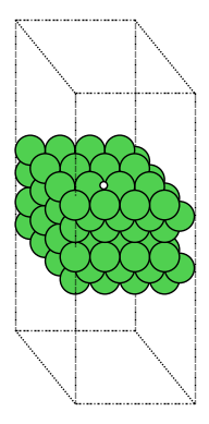

Step 8: Visualize and Compare Results#
Visualize the best configuration and compare with literature:
print("\n7. Visualizing best H* configuration...")
view(slab_with_h, viewer='x3d')
7. Visualizing best H* configuration...
Missing UMA access?
Don’t have access to UMA yet? You can still explore this calculation!
Download example H on Ni(111) structure and test it in the UMA demo (no login required) to see how the model predicts adsorption properties.
# 6. Compare with literature
print(f"\n{'='*60}")
print("Comparison with Literature:")
print(f"{'='*60}")
print("Table 4 (DFT): -0.60 eV (Ni(111), ref H₂)")
print(f"This work:     {E_ads_zpe:.2f} eV")
print(f"Difference:    {abs(E_ads_zpe - (-0.60)):.2f} eV")
============================================================
Comparison with Literature:
============================================================
Table 4 (DFT): -0.60 eV (Ni(111), ref H₂)
This work:     -0.55-0.00j eV
Difference:    0.05 eV
D3 Dispersion Corrections
Dispersion (van der Waals) interactions are important for:
Large molecules (CO, CO₂)
Physisorption
Metal-support interfaces
For H adsorption, D3 corrections are typically small (<0.1 eV) because H forms strong covalent bonds with the surface. However, always check the magnitude!
Explore on Your Own#
Site preference: Identify which site (fcc, hcp, bridge, top) the H prefers. Visualize with
view(atoms, viewer='x3d').Coverage effects: Place 2 H atoms on the slab. How does binding change with separation?
Different facets: Compare H adsorption on (100) and (110) surfaces. Which is strongest?
Subsurface H: Place H below the surface layer. Is it stable?
ZPE uncertainty: How sensitive is E_ads to the vibrational delta parameter (try 0.01, 0.03 Å)?
Part 5: Coverage-Dependent H Adsorption#
Introduction#
At higher coverages, adsorbate-adsorbate interactions become significant. We’ll study how H binding energy changes from dilute (1 atom) to saturated (full monolayer) coverage.
Theory#
The differential adsorption energy at coverage θ is:
For many systems, this varies linearly:
where β quantifies lateral interactions (repulsive if β > 0).
Step 1: Setup Slab and Calculators#
Create a larger Ni(111) slab to accommodate multiple adsorbates:
# Create large Ni(111) slab
ni_bulk_atoms = bulk("Ni", "fcc", a=a_opt, cubic=True)
ni_bulk_obj = Bulk(bulk_atoms=ni_bulk_atoms)
ni_slabs = Slab.from_bulk_get_specific_millers(
    bulk=ni_bulk_obj, specific_millers=(1, 1, 1)
)
slab = ni_slabs[0].atoms.copy()

print(f"   Created {len(slab)} atom slab")

# Set up calculators
base_calc = FAIRChemCalculator(predictor, task_name="oc20")
d3_calc = TorchDFTD3Calculator(device="cpu", damping="bj")
print("   ✓ Calculators initialized")
   Created 96 atom slab
   ✓ Calculators initialized
Step 2: Calculate Reference Energies#
Get reference energies for clean surface and H₂:
print("\n1. Relaxing clean slab...")
clean_slab = slab.copy()
clean_slab.pbc = True
clean_slab.calc = base_calc

opt = LBFGS(
    clean_slab,
    trajectory=str(output_dir / part_dirs["part5"] / "ni111_clean.traj"),
    logfile=str(output_dir / part_dirs["part5"] / "ni111_clean.log"),
)
opt.run(fmax=0.05, steps=relaxation_steps)

E_clean_ml = clean_slab.get_potential_energy()
clean_slab.calc = d3_calc
E_clean_d3 = clean_slab.get_potential_energy()
E_clean = E_clean_ml + E_clean_d3
print(f"   E(clean): {E_clean:.2f} eV")

print("\n2. Calculating H₂ reference...")
h2 = Atoms("H2", positions=[[0, 0, 0], [0, 0, 0.74]])
h2.center(vacuum=10.0)
h2.set_pbc([True, True, True])
h2.calc = base_calc

opt = LBFGS(
    h2,
    trajectory=str(output_dir / part_dirs["part5"] / "h2.traj"),
    logfile=str(output_dir / part_dirs["part5"] / "h2.log"),
)
opt.run(fmax=0.05, steps=relaxation_steps)

E_h2_ml = h2.get_potential_energy()
h2.calc = d3_calc
E_h2_d3 = h2.get_potential_energy()
E_h2 = E_h2_ml + E_h2_d3
print(f"   E(H₂): {E_h2:.2f} eV")
1. Relaxing clean slab...
   E(clean): -487.46 eV

2. Calculating H₂ reference...
   E(H₂): -6.97 eV
Step 3: Set Up Coverage Study#
Define the coverages we’ll test (from dilute to nearly 1 ML):
# Count surface sites
tags = slab.get_tags()
n_sites = np.sum(tags == 1)
print(f"\n3. Surface sites: {n_sites} (4×4 Ni(111))")

# Test coverages: 1 H, 0.25 ML, 0.5 ML, 0.75 ML, 1.0 ML
coverages_to_test = [1, 4, 8, 12, 16]
print(f"\n   Will test coverages: {[f'{n/n_sites:.2f} ML' for n in coverages_to_test]}")
print("   This spans from dilute to nearly full monolayer")

coverages = []
adsorption_energies = []
3. Surface sites: 16 (4×4 Ni(111))

   Will test coverages: ['0.06 ML', '0.25 ML', '0.50 ML', '0.75 ML', '1.00 ML']
   This spans from dilute to nearly full monolayer
Step 4: Generate and Relax Configurations at Each Coverage#
For each coverage, generate multiple configurations and find the lowest energy:
for n_h in coverages_to_test:
    print(f"\n3. Coverage: {n_h} H ({n_h/n_sites:.2f} ML)")

    # Generate configurations
    ni_bulk_obj_h = Bulk(bulk_atoms=ni_bulk_atoms)
    ni_slabs_h = Slab.from_bulk_get_specific_millers(
        bulk=ni_bulk_obj_h, specific_millers=(1, 1, 1)
    )
    slab_for_ads = ni_slabs_h[0]
    slab_for_ads.atoms = clean_slab.copy()

    adsorbates_list = [Adsorbate(adsorbate_smiles_from_db="*H") for _ in range(n_h)]

    try:
        multi_ads_config = MultipleAdsorbateSlabConfig(
            slab_for_ads, adsorbates_list, num_configurations=num_sites
        )
    except ValueError as e:
        print(f"   ⚠ Configuration generation failed: {e}")
        continue

    if len(multi_ads_config.atoms_list) == 0:
        print(f"   ⚠ No configurations generated")
        continue

    print(f"   Generated {len(multi_ads_config.atoms_list)} configurations")

    # Relax each and find best
    config_energies = []

    for idx, config in enumerate(multi_ads_config.atoms_list):
        config_relaxed = config.copy()
        config_relaxed.set_pbc([True, True, True])
        config_relaxed.calc = base_calc

        opt = LBFGS(config_relaxed, logfile=None)
        opt.run(fmax=0.05, steps=relaxation_steps)

        E_ml = config_relaxed.get_potential_energy()
        config_relaxed.calc = d3_calc
        E_d3 = config_relaxed.get_potential_energy()
        E_total = E_ml + E_d3

        config_energies.append(E_total)
        print(f"     Config {idx+1}: {E_total:.2f} eV")

    best_idx = np.argmin(config_energies)
    best_energy = config_energies[best_idx]
    best_config = multi_ads_config.atoms_list[best_idx]
    E_ads_per_h = (best_energy - E_clean - n_h * 0.5 * E_h2) / n_h

    coverage = n_h / n_sites
    coverages.append(coverage)
    adsorption_energies.append(E_ads_per_h)

    print(f"   → E_ads/H: {E_ads_per_h:.2f} eV")

    # Visualize best configuration at this coverage
    print(f"   Visualizing configuration with {n_h} H atoms...")
    view(best_config, viewer='x3d')

print(f"\n✓ Completed coverage study: {len(coverages)} data points")
3. Coverage: 1 H (0.06 ML)
Generated 5 configurations
Config 1: -491.51 eV
Config 2: -491.51 eV
Config 3: -491.51 eV
Config 4: -491.51 eV
     Config 5: -491.53 eV
   → E_ads/H: -0.58 eV
   Visualizing configuration with 1 H atoms...

3. Coverage: 4 H (0.25 ML)
Generated 5 configurations
Config 1: -503.71 eV
Config 2: -503.46 eV
Config 3: -503.68 eV
Config 4: -503.73 eV
     Config 5: -503.73 eV
   → E_ads/H: -0.58 eV
   Visualizing configuration with 4 H atoms...

3. Coverage: 8 H (0.50 ML)
Generated 5 configurations
Config 1: -519.86 eV
Config 2: -519.74 eV
Config 3: -519.60 eV
Config 4: -519.87 eV
     Config 5: -519.38 eV
   → E_ads/H: -0.56 eV
   Visualizing configuration with 8 H atoms...

3. Coverage: 12 H (0.75 ML)
Generated 5 configurations
Config 1: -533.85 eV
Config 2: -535.38 eV
Config 3: -535.23 eV
Config 4: -534.40 eV
     Config 5: -534.45 eV
   → E_ads/H: -0.51 eV
   Visualizing configuration with 12 H atoms...

3. Coverage: 16 H (1.00 ML)
Generated 5 configurations
Config 1: -547.74 eV
Config 2: -550.50 eV
Config 3: -550.45 eV
Config 4: -550.09 eV
     Config 5: -550.89 eV
   → E_ads/H: -0.48 eV
   Visualizing configuration with 16 H atoms...

✓ Completed coverage study: 5 data points
Step 5: Perform Linear Fit#
Fit E_ads vs coverage to extract the slope (lateral interaction strength):
print("\n4. Performing linear fit to coverage dependence...")

# Linear fit
from numpy.polynomial import Polynomial

p = Polynomial.fit(coverages, adsorption_energies, 1)
slope = p.coef[1]
intercept = p.coef[0]

print(f"\n{'='*60}")
print(f"Linear Fit: E_ads = {intercept:.2f} + {slope:.2f}θ (eV)")
print(f"Slope: {slope * 96.485:.1f} kJ/mol per ML")
print(f"Paper: 8.7 kJ/mol per ML")
print(f"{'='*60}")
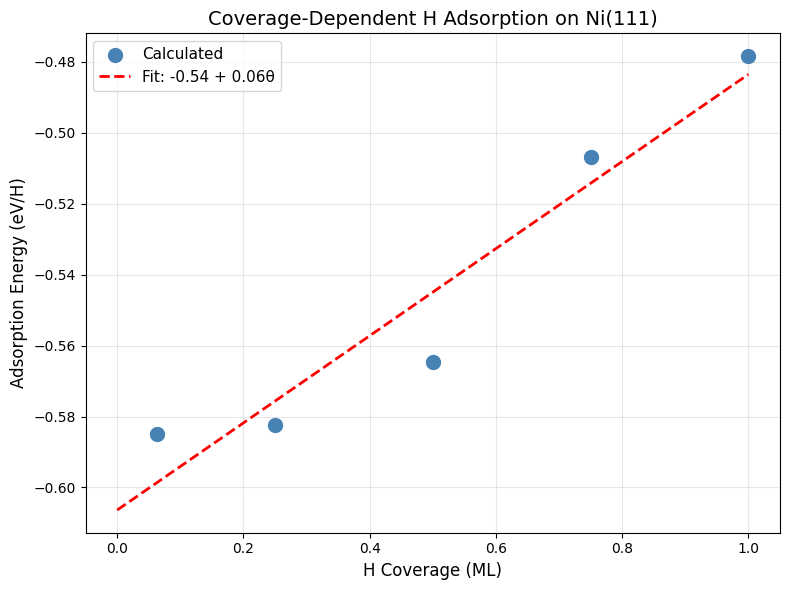
4. Performing linear fit to coverage dependence...

============================================================
Linear Fit: E_ads = -0.54 + 0.06θ (eV)
Slope: 5.6 kJ/mol per ML
Paper: 8.7 kJ/mol per ML
============================================================
Step 6: Visualize Coverage Dependence#
Create a plot showing how adsorption energy changes with coverage:
print("\n5. Plotting coverage dependence...")

# Plot
fig, ax = plt.subplots(figsize=(8, 6))
ax.scatter(
    coverages,
    adsorption_energies,
    s=100,
    marker="o",
    label="Calculated",
    zorder=3,
    color="steelblue",
)

cov_fit = np.linspace(0, max(coverages), 100)
ads_fit = p(cov_fit)
ax.plot(
    cov_fit, ads_fit, "r--", label=f"Fit: {intercept:.2f} + {slope:.2f}θ", linewidth=2
)

ax.set_xlabel("H Coverage (ML)", fontsize=12)
ax.set_ylabel("Adsorption Energy (eV/H)", fontsize=12)
ax.set_title("Coverage-Dependent H Adsorption on Ni(111)", fontsize=14)
ax.legend(fontsize=11)
ax.grid(True, alpha=0.3)
plt.tight_layout()
plt.savefig(str(output_dir / part_dirs["part5"] / "coverage_dependence.png"), dpi=300)
plt.show()

print("\n✓ Coverage dependence analysis complete!")
5. Plotting coverage dependence...
✓ Coverage dependence analysis complete!
Missing UMA access?
Don’t have access to UMA yet? You can still explore this calculation!
Download example multiple H on Ni(111) structure and test it in the UMA demo (no login required) to see how the model handles coverage-dependent binding.
Comparison with Paper
Expected Results from Paper:
Slope: 8.7 kJ/mol per ML (indicating repulsive lateral H-H interactions)
Physical interpretation: H atoms repel weakly due to electrostatic and Pauli effects
What to Check:
Your fitted slope should be close to 8.7 kJ/mol per ML
The relationship should be approximately linear for θ < 1 ML
Intercept (E_ads at θ → 0) should match the single-H result from Part 4 (~-0.60 eV)
Typical Variations:
Slope can vary by ±2-3 kJ/mol depending on slab size and configuration sampling
Non-linearity may appear at very high coverage (θ > 0.75 ML)
Model differences can affect lateral interactions more than adsorption energies
Physical Insights
Positive slope (repulsive interactions):
Electrostatic: H atoms accumulate negative charge from Ni
Pauli repulsion: Overlapping electron clouds
Strain: Lattice distortions propagate
Magnitude:
Weak (~10 kJ/mol/ML) → isolated adsorbates
Strong (>50 kJ/mol/ML) → clustering or phase separation likely
The paper reports 8.7 kJ/mol/ML, indicating relatively weak lateral interactions for H on Ni(111).
Explore on Your Own#
Non-linear behavior: Use polynomial (degree 2) fit. Is there curvature at high coverage?
Temperature effects: Estimate configurational entropy at each coverage. How does this affect free energy?
Pattern formation: Visualize the lowest-energy configuration at 0.5 ML. Are H atoms ordered?
Other adsorbates: Repeat for O or N. How do lateral interactions compare?
Phase diagrams: At what coverage do you expect phase separation (islands vs uniform)?
Part 6: CO Formation/Dissociation Thermochemistry and Barrier#
Introduction#
CO dissociation (CO* → C* + O*) is the rate-limiting step in many catalytic processes (Fischer-Tropsch, CO oxidation, etc.). We’ll calculate the reaction energy for C* + O* → CO* and the activation barriers in both directions using the nudged elastic band (NEB) method.
Theory#
Forward Reaction: C* + O* → CO* + * (recombination)
Reverse Reaction: CO* + → C + O* (dissociation)
Thermochemistry: \(\Delta E_{\text{rxn}} = E(\text{C}^* + \text{O}^*) - E(\text{CO}^*)\)
Barrier: NEB finds the minimum energy path (MEP) and transition state: \(E_a = E^{\ddagger} - E_{\text{initial}}\)
Step 1: Setup Slab and Calculators#
Initialize the Ni(111) surface and calculators:
# Create slab
ni_bulk_atoms = bulk("Ni", "fcc", a=a_opt, cubic=True)
ni_bulk_obj = Bulk(bulk_atoms=ni_bulk_atoms)
ni_slabs = Slab.from_bulk_get_specific_millers(
    bulk=ni_bulk_obj, specific_millers=(1, 1, 1)
)
slab = ni_slabs[0].atoms

print(f"   Created {len(slab)} atom slab")

base_calc = FAIRChemCalculator(predictor, task_name="oc20")
d3_calc = TorchDFTD3Calculator(device="cpu", damping="bj")
print("   \u2713 Calculators initialized")
   Created 96 atom slab
   ✓ Calculators initialized
Step 2: Generate and Relax Final State (CO*)#
Find the most stable CO adsorption configuration (this is the product of C+O recombination):
print("\n1. Final State: CO* on Ni(111)")
print("   Generating CO adsorption configurations...")

ni_bulk_obj_co = Bulk(bulk_atoms=ni_bulk_atoms)
ni_slab_co = Slab.from_bulk_get_specific_millers(
    bulk=ni_bulk_obj_co, specific_millers=(1, 1, 1)
)[0]
ni_slab_co.atoms = slab.copy()

adsorbate_co = Adsorbate(adsorbate_smiles_from_db="*CO")
multi_ads_config_co = MultipleAdsorbateSlabConfig(
    ni_slab_co, [adsorbate_co], num_configurations=num_sites
)

print(f"   Generated {len(multi_ads_config_co.atoms_list)} configurations")

# Relax and find best
co_energies = []
co_energies_ml = []
co_energies_d3 = []
co_configs = []

for idx, config in enumerate(multi_ads_config_co.atoms_list):
    config_relaxed = config.copy()
    config_relaxed.set_pbc([True, True, True])
    config_relaxed.calc = base_calc
    opt = LBFGS(config_relaxed, logfile=None)
    opt.run(fmax=0.05, steps=relaxation_steps)

    E_ml = config_relaxed.get_potential_energy()
    config_relaxed.calc = d3_calc
    E_d3 = config_relaxed.get_potential_energy()
    E_total = E_ml + E_d3

    co_energies.append(E_total)
    co_energies_ml.append(E_ml)
    co_energies_d3.append(E_d3)
    co_configs.append(config_relaxed)
    print(
        f"     Config {idx+1}: E_total = {E_total:.2f} eV (RPBE: {E_ml:.2f}, D3: {E_d3:.2f})"
    )

best_co_idx = np.argmin(co_energies)
final_co = co_configs[best_co_idx]
E_final_co = co_energies[best_co_idx]
E_final_co_ml = co_energies_ml[best_co_idx]
E_final_co_d3 = co_energies_d3[best_co_idx]

print(f"\n   → Best CO* (Config {best_co_idx+1}):")
print(f"      RPBE:  {E_final_co_ml:.2f} eV")
print(f"      D3:    {E_final_co_d3:.2f} eV")
print(f"      Total: {E_final_co:.2f} eV")

# Save best CO state
ase.io.write(str(output_dir / part_dirs["part6"] / "co_final_best.traj"), final_co)
print("   ✓ Best CO* structure saved")

# Visualize best CO* structure
print("\n   Visualizing best CO* structure...")
view(final_co, viewer='x3d')
1. Final State: CO* on Ni(111)
   Generating CO adsorption configurations...
Generated 5 configurations
Config 1: E_total = -503.58 eV (RPBE: -466.73, D3: -36.85)
Config 2: E_total = -503.96 eV (RPBE: -467.14, D3: -36.82)
Config 3: E_total = -503.97 eV (RPBE: -467.14, D3: -36.82)
Config 4: E_total = -503.97 eV (RPBE: -467.14, D3: -36.82)
     Config 5: E_total = -503.97 eV (RPBE: -467.14, D3: -36.82)

   → Best CO* (Config 4):
      RPBE:  -467.14 eV
      D3:    -36.82 eV
      Total: -503.97 eV
   ✓ Best CO* structure saved

   Visualizing best CO* structure...
Step 3: Generate and Relax Initial State (C* + O*)#
Find the most stable configuration for dissociated C and O (reactants):
print("\n2. Initial State: C* + O* on Ni(111)")
print("   Generating C+O configurations...")

ni_bulk_obj_c_o = Bulk(bulk_atoms=ni_bulk_atoms)
ni_slab_c_o = Slab.from_bulk_get_specific_millers(
    bulk=ni_bulk_obj_c_o, specific_millers=(1, 1, 1)
)[0]

adsorbate_c = Adsorbate(adsorbate_smiles_from_db="*C")
adsorbate_o = Adsorbate(adsorbate_smiles_from_db="*O")

multi_ads_config_c_o = MultipleAdsorbateSlabConfig(
    ni_slab_c_o, [adsorbate_c, adsorbate_o], num_configurations=num_sites
)

print(f"   Generated {len(multi_ads_config_c_o.atoms_list)} configurations")

c_o_energies = []
c_o_energies_ml = []
c_o_energies_d3 = []
c_o_configs = []

for idx, config in enumerate(multi_ads_config_c_o.atoms_list):
    config_relaxed = config.copy()
    config_relaxed.set_pbc([True, True, True])
    config_relaxed.calc = base_calc
    opt = LBFGS(config_relaxed, logfile=None)
    opt.run(fmax=0.05, steps=relaxation_steps)

    # Check C-O bond distance to ensure they haven't formed CO molecule
    c_o_dist = config_relaxed[config_relaxed.get_tags() == 2].get_distance(
        0, 1, mic=True
    )

    # CO bond length is ~1.15 Å, so if distance < 1.5 Å, they've formed a molecule
    if c_o_dist < 1.5:
        print(
            f"     Config {idx+1}: ⚠ REJECTED - C and O formed CO molecule (d = {c_o_dist:.2f} Å)"
        )
        continue

    E_ml = config_relaxed.get_potential_energy()
    config_relaxed.calc = d3_calc
    E_d3 = config_relaxed.get_potential_energy()
    E_total = E_ml + E_d3

    c_o_energies.append(E_total)
    c_o_energies_ml.append(E_ml)
    c_o_energies_d3.append(E_d3)
    c_o_configs.append(config_relaxed)
    print(
        f"     Config {idx+1}: E_total = {E_total:.2f} eV (RPBE: {E_ml:.2f}, D3: {E_d3:.2f}, C-O dist: {c_o_dist:.2f} Å)"
    )

best_c_o_idx = np.argmin(c_o_energies)
initial_c_o = c_o_configs[best_c_o_idx]
E_initial_c_o = c_o_energies[best_c_o_idx]
E_initial_c_o_ml = c_o_energies_ml[best_c_o_idx]
E_initial_c_o_d3 = c_o_energies_d3[best_c_o_idx]

print(f"\n   → Best C*+O* (Config {best_c_o_idx+1}):")
print(f"      RPBE:  {E_initial_c_o_ml:.2f} eV")
print(f"      D3:    {E_initial_c_o_d3:.2f} eV")
print(f"      Total: {E_initial_c_o:.2f} eV")

# Save best C+O state
ase.io.write(str(output_dir / part_dirs["part6"] / "co_initial_best.traj"), initial_c_o)
print("   ✓ Best C*+O* structure saved")

# Visualize best C*+O* structure
print("\n   Visualizing best C*+O* structure...")
view(initial_c_o, viewer='x3d')
2. Initial State: C* + O* on Ni(111)
   Generating C+O configurations...
Generated 5 configurations
Config 1: E_total = -502.89 eV (RPBE: -465.98, D3: -36.90, C-O dist: 3.84 Å)
Config 2: E_total = -502.89 eV (RPBE: -465.99, D3: -36.90, C-O dist: 5.18 Å)
Config 3: E_total = -502.49 eV (RPBE: -465.60, D3: -36.89, C-O dist: 2.95 Å)
Config 4: E_total = -502.72 eV (RPBE: -465.83, D3: -36.89, C-O dist: 3.82 Å)
     Config 5: E_total = -502.73 eV (RPBE: -465.84, D3: -36.89, C-O dist: 3.82 Å)

   → Best C*+O* (Config 2):
      RPBE:  -465.99 eV
      D3:    -36.90 eV
      Total: -502.89 eV
   ✓ Best C*+O* structure saved

   Visualizing best C*+O* structure...
Step 3b: Calculate C* and O* Energies Separately#
Another strategy to calculate the initial energies for *C and *O at very low coverage (without interactions between the two reactants) is to do two separate relaxations.
# Clean slab
ni_bulk_obj = Bulk(bulk_atoms=ni_bulk_atoms)
clean_slab = Slab.from_bulk_get_specific_millers(
    bulk=ni_bulk_obj_c_o, specific_millers=(1, 1, 1)
)[0].atoms
clean_slab.set_pbc([True, True, True])
clean_slab.calc = base_calc
opt = LBFGS(clean_slab, logfile=None)
opt.run(fmax=0.05, steps=relaxation_steps)

E_clean_ml = clean_slab.get_potential_energy()
clean_slab.calc = d3_calc
E_clean_d3 = clean_slab.get_potential_energy()
E_clean = E_clean_ml + E_clean_d3

print(
    f"\n   Clean slab: E_total = {E_clean:.2f} eV (RPBE: {E_clean_ml:.2f}, D3: {E_clean_d3:.2f})"
)
Clean slab: E_total = -487.46 eV (RPBE: -450.89, D3: -36.57)
print(f"\n2b. Separate C* and O* Energies:")
print("    Calculating energies in separate unit cells to avoid interactions")

ni_bulk_obj_c_o = Bulk(bulk_atoms=ni_bulk_atoms)
ni_slab_c_o = Slab.from_bulk_get_specific_millers(
    bulk=ni_bulk_obj_c_o, specific_millers=(1, 1, 1)
)[0]

print("\n   Generating C* configurations...")
multi_ads_config_c = MultipleAdsorbateSlabConfig(
    ni_slab_c_o,
    adsorbates=[Adsorbate(adsorbate_smiles_from_db="*C")],
    num_configurations=num_sites,
)

c_energies = []
c_energies_ml = []
c_energies_d3 = []
c_configs = []

for idx, config in enumerate(multi_ads_config_c.atoms_list):
    config_relaxed = config.copy()
    config_relaxed.set_pbc([True, True, True])
    config_relaxed.calc = base_calc
    opt = LBFGS(config_relaxed, logfile=None)
    opt.run(fmax=0.05, steps=relaxation_steps)

    E_ml = config_relaxed.get_potential_energy()
    config_relaxed.calc = d3_calc
    E_d3 = config_relaxed.get_potential_energy()
    E_total = E_ml + E_d3

    c_energies.append(E_total)
    c_energies_ml.append(E_ml)
    c_energies_d3.append(E_d3)
    c_configs.append(config_relaxed)
    print(
        f"     Config {idx+1}: E_total = {E_total:.2f} eV (RPBE: {E_ml:.2f}, D3: {E_d3:.2f})"
    )

best_c_idx = np.argmin(c_energies)
c_ads = c_configs[best_c_idx]
E_c = c_energies[best_c_idx]
E_c_ml = c_energies_ml[best_c_idx]
E_c_d3 = c_energies_d3[best_c_idx]

print(f"\n   → Best C* (Config {best_c_idx+1}):")
print(f"      RPBE:  {E_c_ml:.2f} eV")
print(f"      D3:    {E_c_d3:.2f} eV")
print(f"      Total: {E_c:.2f} eV")

# Save best C state
ase.io.write(str(output_dir / part_dirs["part6"] / "c_best.traj"), c_ads)

# Visualize best C* structure
print("\n   Visualizing best C* structure...")
view(c_ads, viewer='x3d')

# Generate O* configuration
print("\n   Generating O* configurations...")
multi_ads_config_o = MultipleAdsorbateSlabConfig(
    ni_slab_c_o,
    adsorbates=[Adsorbate(adsorbate_smiles_from_db="*O")],
    num_configurations=num_sites,
)
o_energies = []
o_energies_ml = []
o_energies_d3 = []
o_configs = []

for idx, config in enumerate(multi_ads_config_o.atoms_list):
    config_relaxed = config.copy()
    config_relaxed.set_pbc([True, True, True])
    config_relaxed.calc = base_calc
    opt = LBFGS(config_relaxed, logfile=None)
    opt.run(fmax=0.05, steps=relaxation_steps)

    E_ml = config_relaxed.get_potential_energy()
    config_relaxed.calc = d3_calc
    E_d3 = config_relaxed.get_potential_energy()
    E_total = E_ml + E_d3

    o_energies.append(E_total)
    o_energies_ml.append(E_ml)
    o_energies_d3.append(E_d3)
    o_configs.append(config_relaxed)
    print(
        f"     Config {idx+1}: E_total = {E_total:.2f} eV (RPBE: {E_ml:.2f}, D3: {E_d3:.2f})"
    )

best_o_idx = np.argmin(o_energies)
o_ads = o_configs[best_o_idx]
E_o = o_energies[best_o_idx]
E_o_ml = o_energies_ml[best_o_idx]
E_o_d3 = o_energies_d3[best_o_idx]

print(f"\n   → Best O* (Config {best_o_idx+1}):")
print(f"      RPBE:  {E_o_ml:.2f} eV")
print(f"      D3:    {E_o_d3:.2f} eV")
print(f"      Total: {E_o:.2f} eV")

# Save best O state
ase.io.write(str(output_dir / part_dirs["part6"] / "o_best.traj"), o_ads)

# Visualize best O* structure
print("\n   Visualizing best O* structure...")
view(o_ads, viewer='x3d')

# Calculate combined energy for separate C* and O*
E_initial_c_o_separate = E_c + E_o
E_initial_c_o_separate_ml = E_c_ml + E_o_ml
E_initial_c_o_separate_d3 = E_c_d3 + E_o_d3
2b. Separate C* and O* Energies:
    Calculating energies in separate unit cells to avoid interactions
Generating C* configurations...
Config 1: E_total = -495.66 eV (RPBE: -458.89, D3: -36.77)
Config 2: E_total = -495.71 eV (RPBE: -458.93, D3: -36.78)
Config 3: E_total = -495.67 eV (RPBE: -458.89, D3: -36.77)
Config 4: E_total = -495.67 eV (RPBE: -458.89, D3: -36.78)
     Config 5: E_total = -495.73 eV (RPBE: -458.94, D3: -36.78)

   → Best C* (Config 5):
      RPBE:  -458.94 eV
      D3:    -36.78 eV
      Total: -495.73 eV

   Visualizing best C* structure...

   Generating O* configurations...
Config 1: E_total = -494.55 eV (RPBE: -457.87, D3: -36.68)
Config 2: E_total = -494.66 eV (RPBE: -457.97, D3: -36.68)
Config 3: E_total = -494.66 eV (RPBE: -457.97, D3: -36.69)
Config 4: E_total = -494.55 eV (RPBE: -457.87, D3: -36.68)
     Config 5: E_total = -494.56 eV (RPBE: -457.87, D3: -36.68)

   → Best O* (Config 3):
      RPBE:  -457.97 eV
      D3:    -36.69 eV
      Total: -494.66 eV

   Visualizing best O* structure...
print(f"\n   Combined C* + O* (separate calculations):")
print(f"      RPBE:  {E_initial_c_o_separate_ml:.2f} eV")
print(f"      D3:    {E_initial_c_o_separate_d3:.2f} eV")
print(f"      Total: {E_initial_c_o_separate:.2f} eV")

print(f"\n   Comparison:")
print(f"      C*+O* (same cell):  {E_initial_c_o - E_clean:.2f} eV")
print(f"      C* + O* (separate): {E_initial_c_o_separate - 2*E_clean:.2f} eV")
print(
    f"      Difference:         {(E_initial_c_o - E_clean) - (E_initial_c_o_separate - 2*E_clean):.2f} eV"
)
print("   ✓ Separate C* and O* energies calculated")
   Combined C* + O* (separate calculations):
      RPBE:  -916.91 eV
      D3:    -73.47 eV
      Total: -990.38 eV

   Comparison:
      C*+O* (same cell):  -15.43 eV
      C* + O* (separate): -15.46 eV
      Difference:         0.03 eV
   ✓ Separate C* and O* energies calculated
Step 4: Calculate Reaction Energy with ZPE#
Compute the thermochemistry for C* + O* → CO* with ZPE corrections:
print(f"\n3. Reaction Energy (C* + O* → CO*):")
print(f"   " + "=" * 60)

# Electronic energies
print(f"\n   Electronic Energies:")
print(
    f"   Initial (C*+O*): RPBE = {E_initial_c_o_ml:.2f} eV, D3 = {E_initial_c_o_d3:.2f} eV, Total = {E_initial_c_o:.2f} eV"
)
print(
    f"   Final (CO*):     RPBE = {E_final_co_ml:.2f} eV, D3 = {E_final_co_d3:.2f} eV, Total = {E_final_co:.2f} eV"
)

# Reaction energies without ZPE
delta_E_rpbe = E_final_co_ml - E_initial_c_o_ml
delta_E_d3_contrib = E_final_co_d3 - E_initial_c_o_d3
delta_E_elec = E_final_co - E_initial_c_o

print(f"\n   Reaction Energies (without ZPE):")
print(f"   ΔE(RPBE only):     {delta_E_rpbe:.2f} eV = {delta_E_rpbe*96.485:.1f} kJ/mol")
print(
    f"   ΔE(D3 contrib):    {delta_E_d3_contrib:.2f} eV = {delta_E_d3_contrib*96.485:.1f} kJ/mol"
)
print(f"   ΔE(RPBE+D3):       {delta_E_elec:.2f} eV = {delta_E_elec*96.485:.1f} kJ/mol")

# Calculate ZPE for CO* (final state)
print(f"\n   Computing ZPE for CO*...")
final_co.calc = base_calc

co_indices = np.where(final_co.get_tags() == 2)[0]
vib_co = Vibrations(final_co, indices=co_indices, delta=0.02, name="vib_co")
vib_co.run()
vib_energies_co = vib_co.get_energies()
zpe_co = np.sum(vib_energies_co[vib_energies_co > 0]) / 2.0
vib_co.clean()
print(f"   ZPE(CO*): {zpe_co:.2f} eV ({zpe_co*1000:.1f} meV)")


# Calculate ZPE for C* and O* (initial state)
print(f"\n   Computing ZPE for C* and O*...")
initial_c_o.calc = base_calc
c_o_indices = np.where(initial_c_o.get_tags() == 2)[0]
vib_c_o = Vibrations(initial_c_o, indices=c_o_indices, delta=0.02, name="vib_c_o")
vib_c_o.run()
vib_energies_c_o = vib_c_o.get_energies()
zpe_c_o = np.sum(vib_energies_c_o[vib_energies_c_o > 0]) / 2.0
vib_c_o.clean()
print(f"   ZPE(C*+O*): {zpe_c_o:.2f} eV ({zpe_c_o*1000:.1f} meV)")


# Total reaction energy with ZPE
delta_zpe = zpe_co - zpe_c_o
delta_E_zpe = delta_E_elec + delta_zpe

print(f"\n   Reaction Energy (with ZPE):")
print(f"   ΔE(electronic):    {delta_E_elec:.2f} eV = {delta_E_elec*96.485:.1f} kJ/mol")
print(
    f"   ΔZPE:              {delta_zpe:.2f} eV = {delta_zpe*96.485:.1f} kJ/mol ({delta_zpe*1000:.1f} meV)"
)
print(f"   ΔE(total):         {delta_E_zpe:.2f} eV = {delta_E_zpe*96.485:.1f} kJ/mol")

print(f"\n   Summary:")
print(
    f"   Without D3, without ZPE: {delta_E_rpbe:.2f} eV = {delta_E_rpbe*96.485:.1f} kJ/mol"
)
print(
    f"   With D3, without ZPE:    {delta_E_elec:.2f} eV = {delta_E_elec*96.485:.1f} kJ/mol"
)
print(
    f"   With D3, with ZPE:       {delta_E_zpe:.2f} eV = {delta_E_zpe*96.485:.1f} kJ/mol"
)

print(f"\n   " + "=" * 60)
print(f"\n   Comparison with Paper (Table 5):")
print(f"   Paper (DFT-D3): -142.7 kJ/mol = -1.48 eV")
print(f"   This work:      {delta_E_zpe*96.485:.1f} kJ/mol = {delta_E_zpe:.2f} eV")
print(f"   Difference:     {abs(delta_E_zpe - (-1.48)):.2f} eV")

if delta_E_zpe < 0:
    print(f"\n   ✓ Reaction is exothermic (C+O recombination favorable)")
else:
    print(f"\n   ⚠ Reaction is endothermic (dissociation favorable)")
3. Reaction Energy (C* + O* → CO*):
   ============================================================

   Electronic Energies:
   Initial (C*+O*): RPBE = -465.99 eV, D3 = -36.90 eV, Total = -502.89 eV
   Final (CO*):     RPBE = -467.14 eV, D3 = -36.82 eV, Total = -503.97 eV

   Reaction Energies (without ZPE):
   ΔE(RPBE only):     -1.16 eV = -111.5 kJ/mol
   ΔE(D3 contrib):    0.08 eV = 7.3 kJ/mol
   ΔE(RPBE+D3):       -1.08 eV = -104.2 kJ/mol

   Computing ZPE for CO*...
   ZPE(CO*): 0.18+0.00j eV (182.9+0.0j meV)

   Computing ZPE for C* and O*...
   ZPE(C*+O*): 0.18+0.00j eV (175.9+0.0j meV)

   Reaction Energy (with ZPE):
   ΔE(electronic):    -1.08 eV = -104.2 kJ/mol
   ΔZPE:              0.01+0.00j eV = 0.7+0.0j kJ/mol (6.9+0.0j meV)
   ΔE(total):         -1.07+0.00j eV = -103.5+0.0j kJ/mol

   Summary:
   Without D3, without ZPE: -1.16 eV = -111.5 kJ/mol
   With D3, without ZPE:    -1.08 eV = -104.2 kJ/mol
   With D3, with ZPE:       -1.07+0.00j eV = -103.5+0.0j kJ/mol

   ============================================================

   Comparison with Paper (Table 5):
   Paper (DFT-D3): -142.7 kJ/mol = -1.48 eV
   This work:      -103.5+0.0j kJ/mol = -1.07+0.00j eV
   Difference:     0.41 eV

   ✓ Reaction is exothermic (C+O recombination favorable)
Step 5: Calculate CO Adsorption Energy (Bonus)#
Calculate how strongly CO binds to the surface:
print(f"\n4. CO Adsorption Energy ( CO(g) + * → CO*):")
print("   This helps us understand CO binding strength")

# CO(g)
co_gas = Atoms("CO", positions=[[0, 0, 0], [0, 0, 1.15]])
co_gas.center(vacuum=10.0)
co_gas.set_pbc([True, True, True])
co_gas.calc = base_calc
opt = LBFGS(co_gas, logfile=None)
opt.run(fmax=0.05, steps=relaxation_steps)

E_co_gas_ml = co_gas.get_potential_energy()
co_gas.calc = d3_calc
E_co_gas_d3 = co_gas.get_potential_energy()
E_co_gas = E_co_gas_ml + E_co_gas_d3

print(
    f"   CO(g):       E_total = {E_co_gas:.2f} eV (RPBE: {E_co_gas_ml:.2f}, D3: {E_co_gas_d3:.2f})"
)

# Calculate ZPE for CO(g)
co_gas.calc = base_calc
vib_co_gas = Vibrations(co_gas, indices=[0, 1], delta=0.01, nfree=2)
vib_co_gas.clean()
vib_co_gas.run()
vib_energies_co_gas = vib_co_gas.get_energies()
zpe_co_gas = 0.5 * np.sum(vib_energies_co_gas[vib_energies_co_gas > 0])
vib_co_gas.clean()

print(f"   ZPE(CO(g)):  {zpe_co_gas:.2f} eV")
print(f"   ZPE(CO*):    {zpe_co:.2f} eV (from Step 4 calculation)")

# Electronic adsorption energy
E_ads_co_elec = E_final_co - E_clean - E_co_gas

# ZPE contribution to adsorption energy
delta_zpe_ads = zpe_co - zpe_co_gas

# Total adsorption energy with ZPE
E_ads_co_total = E_ads_co_elec + delta_zpe_ads

print(f"\n   Electronic Energy Breakdown:")
print(f"   ΔE(RPBE only) = {(E_final_co_ml - E_clean_ml - E_co_gas_ml):.2f} eV")
print(f"   ΔE(D3 contrib) = {((E_final_co_d3 - E_clean_d3 - E_co_gas_d3)):.2f} eV")
print(f"   ΔE(RPBE+D3) = {E_ads_co_elec:.2f} eV")
print(f"\n   ZPE Contribution:")
print(f"   ΔZPE = {delta_zpe_ads:.2f} eV")
print(f"\n   Total Adsorption Energy:")
print(f"   ΔE(total) = {E_ads_co_total:.2f} eV = {E_ads_co_total*96.485:.1f} kJ/mol")
print(f"\n   Summary:")
print(
    f"   E_ads(CO) without ZPE = {-E_ads_co_elec:.2f} eV = {-E_ads_co_elec*96.485:.1f} kJ/mol"
)
print(
    f"   E_ads(CO) with ZPE    = {-E_ads_co_total:.2f} eV = {-E_ads_co_total*96.485:.1f} kJ/mol"
)
print(
    f"   → CO binds {abs(E_ads_co_total):.2f} eV stronger than H ({abs(E_ads_co_total)/0.60:.1f}x)"
)
4. CO Adsorption Energy ( CO(g) + * → CO*):
   This helps us understand CO binding strength
CO(g): E_total = -14.43 eV (RPBE: -14.42, D3: -0.01)
   ZPE(CO(g)):  0.13+0.00j eV
   ZPE(CO*):    0.18+0.00j eV (from Step 4 calculation)

   Electronic Energy Breakdown:
   ΔE(RPBE only) = -1.84 eV
   ΔE(D3 contrib) = -0.24 eV
   ΔE(RPBE+D3) = -2.08 eV

   ZPE Contribution:
   ΔZPE = 0.05-0.00j eV

   Total Adsorption Energy:
   ΔE(total) = -2.03-0.00j eV = -195.6-0.0j kJ/mol

   Summary:
   E_ads(CO) without ZPE = 2.08 eV = 200.5 kJ/mol
   E_ads(CO) with ZPE    = 2.03+0.00j eV = 195.6+0.0j kJ/mol
   → CO binds 2.03 eV stronger than H (3.4x)
Comparison with Paper Results
The paper reports a CO adsorption energy of 1.82 eV (175.6 kJ/mol) in Table 4, calculated using DFT (RPBE functional).
These results show:
Without ZPE: The electronic binding energy matches well with DFT predictions
With ZPE: The zero-point energy correction reduces the binding strength slightly
D3 Dispersion: Contributes to stronger binding due to van der Waals interactions
Step 6: Find guesses for nearby initial and final states for the reaction#
Now that we have an estimate on the reaction energy from the best possible initial and final states, we want to find a transition state (barrier) for this reaction. There are MANY possible ways that we could do this. In this case, we’ll start with the *CO final state and then try and find a nearby local minimal of *C and *O, by fixing the C-O bond distance and finding a nearby local minima. Note that this approach required some insight into what the transition state might look like, and could be considerably more complicated for a reaction that did not involve breaking a single bond.
print(f"\nFinding Transition State Initial and Final States")
print("   Creating initial guess with stretched C-O bond...")
print("   Starting from CO* and stretching the C-O bond...")

# Create a guess structure with stretched CO bond (start from CO*)
initial_guess = final_co.copy()

# Set up a constraint to fix the bond length to ~2 Angstroms, which should be far enough that we'll be closer to *C+*O than *CO
co_indices = np.where(initial_guess.get_tags() == 2)[0]

# Rotate the atoms a bit just to break the symmetry and prevent the O from going straight up to satisfy the constraint
initial_slab = initial_guess[initial_guess.get_tags() != 2]
initial_co = initial_guess[initial_guess.get_tags() == 2]
initial_co.rotate(30, "x", center=initial_co.positions[0])
initial_guess = initial_slab + initial_co

initial_guess.calc = FAIRChemCalculator(predictor, task_name="oc20")

# Add constraints to keep the CO bond length extended
initial_guess.constraints += [
    FixBondLengths([co_indices], tolerance=1e-2, iterations=5000, bondlengths=[2.0])
]


try:
    opt = LBFGS(
        initial_guess,
        trajectory=output_dir / part_dirs["part6"] / "initial_guess_with_constraint.traj",
    )
    opt.run(fmax=0.01)
except RuntimeError:
    # The FixBondLength constraint is sometimes a little finicky,
    # but it's ok if it doesn't finish as it's just an initial guess
    # for the next step
    pass

# Now that we have a guess, re-relax without the constraints
initial_guess.constraints = initial_guess.constraints[:-1]
opt = LBFGS(
    initial_guess,
    trajectory=output_dir
    / part_dirs["part6"]
    / "initial_guess_without_constraint.traj",
)
opt.run(fmax=0.01)
Finding Transition State Initial and Final States
   Creating initial guess with stretched C-O bond...
   Starting from CO* and stretching the C-O bond...
       Step     Time          Energy          fmax
LBFGS:    0 23:01:51     -466.820814        0.933386
LBFGS: 1 23:01:52 -461.473533 4.201399
LBFGS: 2 23:01:52 -461.541569 3.819022
LBFGS: 3 23:01:52 -461.870045 0.990589
LBFGS: 4 23:01:52 -461.937244 0.981921
LBFGS: 5 23:01:52 -461.962917 0.956283
LBFGS: 6 23:01:52 -461.954811 0.755221
LBFGS: 7 23:01:53 -462.007534 0.444253
LBFGS: 8 23:01:53 -461.961218 0.403348
LBFGS: 9 23:01:53 -462.022161 1.000305
LBFGS: 10 23:01:53 -462.031080 0.415334
LBFGS: 11 23:01:53 -462.046242 0.494780
LBFGS: 12 23:01:54 -462.085886 0.663025
LBFGS: 13 23:01:54 -462.161575 1.372185
LBFGS: 14 23:01:54 -462.215290 1.927856
LBFGS: 15 23:01:54 -462.263727 2.370239
LBFGS: 16 23:01:54 -462.341347 3.287233
LBFGS: 17 23:01:55 -462.304025 3.993962
LBFGS: 18 23:01:55 -462.370334 3.819039
LBFGS: 19 23:01:55 -462.478641 3.378005
LBFGS: 20 23:01:55 -462.646381 2.570744
LBFGS: 21 23:01:55 -462.936364 0.888155
LBFGS: 22 23:01:55 -462.968499 0.692334
LBFGS: 23 23:01:56 -462.997117 0.657991
LBFGS: 24 23:01:56 -463.056911 0.824350
LBFGS: 25 23:01:56 -463.096682 0.662722
LBFGS: 26 23:01:56 -463.107582 0.417180
LBFGS: 27 23:01:56 -463.109198 0.332080
LBFGS: 28 23:01:57 -463.141987 0.453317
LBFGS: 29 23:01:57 -463.165894 0.603940
LBFGS: 30 23:01:57 -463.165788 0.368804
LBFGS: 31 23:01:57 -463.200312 0.322940
LBFGS: 32 23:01:57 -463.208141 0.427666
LBFGS: 33 23:01:58 -463.222295 0.347186
LBFGS: 34 23:01:58 -463.251592 0.350275
LBFGS: 35 23:01:58 -463.240187 0.542475
LBFGS: 36 23:01:58 -463.252578 0.679913
LBFGS: 37 23:01:58 -463.289138 0.325561
LBFGS: 38 23:01:58 -463.296719 0.405574
LBFGS: 39 23:01:59 -463.301332 0.327242
LBFGS: 40 23:01:59 -463.310212 0.394633
LBFGS: 41 23:01:59 -463.342774 0.684987
LBFGS: 42 23:01:59 -463.396908 1.041083
LBFGS: 43 23:01:59 -463.432366 1.025362
LBFGS: 44 23:02:00 -463.502002 0.867384
LBFGS: 45 23:02:00 -463.554373 0.723542
LBFGS: 46 23:02:00 -463.617417 0.567341
LBFGS: 47 23:02:00 -463.638478 0.463407
LBFGS: 48 23:02:00 -463.702004 0.548109
LBFGS: 49 23:02:01 -463.751232 0.413914
LBFGS: 50 23:02:01 -463.804469 0.561162
LBFGS: 51 23:02:01 -463.828709 0.416286
LBFGS: 52 23:02:01 -463.866520 0.462146
LBFGS: 53 23:02:01 -463.927231 0.628401
LBFGS: 54 23:02:01 -463.985978 0.724530
LBFGS: 55 23:02:02 -464.037638 0.610976
LBFGS: 56 23:02:02 -464.063912 0.333690
LBFGS: 57 23:02:02 -464.066657 0.353587
LBFGS: 58 23:02:02 -464.083860 0.260285
LBFGS: 59 23:02:02 -464.110672 0.264590
LBFGS: 60 23:02:03 -464.119084 0.341915
LBFGS: 61 23:02:03 -464.126754 0.208025
LBFGS: 62 23:02:03 -464.129827 0.172884
LBFGS: 63 23:02:03 -464.129852 0.139661
LBFGS: 64 23:02:03 -464.140665 0.269152
LBFGS: 65 23:02:04 -464.140896 0.190554
LBFGS: 66 23:02:04 -464.145262 0.086952
LBFGS: 67 23:02:04 -464.148369 0.099588
LBFGS: 68 23:02:04 -464.150273 0.092913
LBFGS: 69 23:02:04 -464.157723 0.143432
LBFGS: 70 23:02:05 -464.155240 0.129300
LBFGS: 71 23:02:05 -464.155970 0.096974
LBFGS: 72 23:02:05 -464.160528 0.079164
LBFGS: 73 23:02:05 -464.158362 0.064338
LBFGS: 74 23:02:05 -464.158756 0.065502
LBFGS: 75 23:02:05 -464.153729 0.112244
LBFGS: 76 23:02:06 -464.160126 0.100987
LBFGS: 77 23:02:06 -464.157697 0.089216
LBFGS: 78 23:02:06 -464.158551 0.053670
LBFGS: 79 23:02:06 -464.152687 0.089649
LBFGS: 80 23:02:06 -464.160678 0.062396
LBFGS: 81 23:02:07 -464.163423 0.044126
LBFGS: 82 23:02:07 -464.159690 0.029514
LBFGS: 83 23:02:07 -464.157348 0.048974
LBFGS: 84 23:02:07 -464.160700 0.030442
LBFGS: 85 23:02:07 -464.163510 0.048193
LBFGS: 86 23:02:08 -464.164165 0.043521
LBFGS: 87 23:02:08 -464.161469 0.011285
LBFGS: 88 23:02:08 -464.156125 0.068748
LBFGS: 89 23:02:08 -464.160933 0.020223
LBFGS: 90 23:02:08 -464.163947 0.046041
LBFGS: 91 23:02:08 -464.159317 0.031542
LBFGS: 92 23:02:09 -464.159557 0.022492
LBFGS: 93 23:02:09 -464.161383 0.009039
       Step     Time          Energy          fmax
LBFGS:    0 23:02:09     -464.161383        0.471430
LBFGS: 1 23:02:09 -464.167315 0.444832
LBFGS: 2 23:02:09 -464.194849 0.877090
LBFGS: 3 23:02:09 -464.207762 0.494773
LBFGS: 4 23:02:10 -464.229632 0.356215
LBFGS: 5 23:02:10 -464.253263 0.423533
LBFGS: 6 23:02:10 -464.260134 0.331348
LBFGS: 7 23:02:10 -464.272953 0.265914
LBFGS: 8 23:02:10 -464.277216 0.242685
LBFGS: 9 23:02:11 -464.286119 0.165645
LBFGS: 10 23:02:11 -464.287936 0.100330
LBFGS: 11 23:02:11 -464.288964 0.086082
LBFGS: 12 23:02:11 -464.289786 0.095618
LBFGS: 13 23:02:11 -464.290871 0.098506
LBFGS: 14 23:02:11 -464.291574 0.073742
LBFGS: 15 23:02:12 -464.291964 0.049766
LBFGS: 16 23:02:12 -464.292238 0.065252
LBFGS: 17 23:02:12 -464.292587 0.072632
LBFGS: 18 23:02:12 -464.292991 0.059704
LBFGS: 19 23:02:12 -464.293318 0.051375
LBFGS: 20 23:02:13 -464.293476 0.025542
LBFGS: 21 23:02:13 -464.293566 0.023366
LBFGS: 22 23:02:13 -464.293650 0.035601
LBFGS: 23 23:02:13 -464.293746 0.036481
LBFGS: 24 23:02:13 -464.293818 0.023637
LBFGS: 25 23:02:14 -464.293866 0.019519
LBFGS: 26 23:02:14 -464.293916 0.021564
LBFGS: 27 23:02:14 -464.293969 0.031235
LBFGS: 28 23:02:14 -464.294028 0.029366
LBFGS: 29 23:02:14 -464.294075 0.024783
LBFGS: 30 23:02:14 -464.294103 0.023861
LBFGS: 31 23:02:15 -464.294141 0.022086
LBFGS: 32 23:02:15 -464.294195 0.036887
LBFGS: 33 23:02:15 -464.294296 0.047130
LBFGS: 34 23:02:15 -464.294437 0.044491
LBFGS: 35 23:02:15 -464.294647 0.051414
LBFGS: 36 23:02:16 -464.295011 0.068575
LBFGS: 37 23:02:16 -464.296023 0.173091
LBFGS: 38 23:02:16 -464.297490 0.775443
LBFGS: 39 23:02:16 -464.303005 0.811966
LBFGS: 40 23:02:16 -464.330631 1.432142
LBFGS: 41 23:02:17 -464.322623 1.829715
LBFGS: 42 23:02:17 -464.352593 1.414404
LBFGS: 43 23:02:17 -464.362733 1.489075
LBFGS: 44 23:02:17 -464.372667 1.817561
LBFGS: 45 23:02:17 -464.425881 1.464157
LBFGS: 46 23:02:17 -464.459555 1.263348
LBFGS: 47 23:02:18 -464.560936 0.668764
LBFGS: 48 23:02:18 -464.594140 0.595100
LBFGS: 49 23:02:18 -464.633769 0.645798
LBFGS: 50 23:02:18 -464.725106 0.749075
LBFGS: 51 23:02:18 -464.823785 0.942669
LBFGS: 52 23:02:19 -464.881071 1.113297
LBFGS: 53 23:02:19 -464.974202 0.926375
LBFGS: 54 23:02:19 -465.146520 2.045392
LBFGS: 55 23:02:19 -465.261815 1.467569
LBFGS: 56 23:02:19 -465.376877 0.650051
LBFGS: 57 23:02:20 -465.423005 0.677521
LBFGS: 58 23:02:20 -465.477948 0.745277
LBFGS: 59 23:02:20 -465.520185 0.657982
LBFGS: 60 23:02:20 -465.552844 0.393566
LBFGS: 61 23:02:20 -465.564501 0.203771
LBFGS: 62 23:02:20 -465.572925 0.170368
LBFGS: 63 23:02:21 -465.583972 0.138309
LBFGS: 64 23:02:21 -465.588649 0.111978
LBFGS: 65 23:02:21 -465.591139 0.124916
LBFGS: 66 23:02:21 -465.592877 0.107882
LBFGS: 67 23:02:21 -465.594423 0.075868
LBFGS: 68 23:02:22 -465.595598 0.057126
LBFGS: 69 23:02:22 -465.596316 0.038663
LBFGS: 70 23:02:22 -465.596650 0.038949
LBFGS: 71 23:02:22 -465.596886 0.038541
LBFGS: 72 23:02:22 -465.597143 0.049297
LBFGS: 73 23:02:23 -465.597385 0.045003
LBFGS: 74 23:02:23 -465.597557 0.027272
LBFGS: 75 23:02:23 -465.597653 0.020970
LBFGS: 76 23:02:23 -465.597718 0.017150
LBFGS: 77 23:02:23 -465.597795 0.018827
LBFGS: 78 23:02:23 -465.597875 0.016676
LBFGS: 79 23:02:24 -465.597947 0.014520
LBFGS: 80 23:02:24 -465.597982 0.011108
LBFGS: 81 23:02:24 -465.598004 0.009587
np.True_
Step 7: Run NEB to Find Activation Barrier#
Use the nudged elastic band method to find the minimum energy path:
print(f"\n7. NEB Barrier Calculation (C* + O* → CO*)")
print("   Setting up 7-image NEB chain with TS guess in middle...")
print("   Reaction: C* + O* (initial) → TS → CO* (final)")

initial = initial_guess.copy()
initial.calc = FAIRChemCalculator(predictor, task_name="oc20")
images = [initial]  # Start with C* + O*

n_images = 10
for i in range(n_images):
    image = initial.copy()
    image.calc = FAIRChemCalculator(predictor, task_name="oc20")
    images.append(image)

final = final_co.copy()
final.calc = FAIRChemCalculator(predictor, task_name="oc20")
images.append(final)  # End with CO*

# Interpolate with better initial guess
dyneb = DyNEB(images, climb=True, fmax=0.05)

# Interpolate first half (C*+O* → TS)
print("\n   Interpolating images...")
dyneb.interpolate("idpp", mic=True)

# Optimize
print("   Optimizing NEB path (this may take a while)...")
opt = FIRE(
    dyneb,
    trajectory=str(output_dir / part_dirs["part6"] / "neb.traj"),
    logfile=str(output_dir / part_dirs["part6"] / "neb.log"),
)
opt.run(fmax=0.1, steps=relaxation_steps)

# Extract barrier (from C*+O* to TS)
energies = [img.get_potential_energy() for img in images]
energies_rel = np.array(energies) - energies[0]
E_barrier = np.max(energies_rel)

print(f"\n   ✓ NEB converged!")
print(
    f"\n   Forward barrier (C*+O* → CO*): {E_barrier:.2f} eV = {E_barrier*96.485:.1f} kJ/mol"
)
print(
    f"   Reverse barrier (CO* → C*+O*): {E_barrier - energies_rel[-1]:.2f} eV = {(E_barrier- energies_rel[-1])*96.485:.1f} kJ/mol"
)
print(f"\n   Paper (Table 5): 153 kJ/mol = 1.59 eV ")
print(f"   Difference: {abs(E_barrier - 1.59):.2f} eV")
7. NEB Barrier Calculation (C* + O* → CO*)
   Setting up 7-image NEB chain with TS guess in middle...
   Reaction: C* + O* (initial) → TS → CO* (final)

   Interpolating images...
Optimizing NEB path (this may take a while)...
   ✓ NEB converged!

   Forward barrier (C*+O* → CO*): 1.37 eV = 132.2 kJ/mol
   Reverse barrier (CO* → C*+O*): 2.91 eV = 281.2 kJ/mol

   Paper (Table 5): 153 kJ/mol = 1.59 eV
   Difference: 0.22 eV
Step 8: Visualize NEB Path and Key Structures#
Create plots showing the reaction pathway:
print("\n   Creating NEB visualization...")

# Plot NEB path
fig, ax = plt.subplots(figsize=(10, 6))
ax.plot(
    range(len(energies_rel)),
    energies_rel,
    "o-",
    linewidth=2,
    markersize=10,
    color="steelblue",
    label="NEB Path",
)
ax.axhline(0, color="green", linestyle="--", alpha=0.5, label="Initial: C*+O*")
ax.axhline(delta_E_zpe, color="red", linestyle="--", alpha=0.5, label="Final: CO*")
ax.axhline(
    E_barrier,
    color="orange",
    linestyle=":",
    alpha=0.7,
    linewidth=2,
    label=f"Forward Barrier = {E_barrier:.2f} eV",
)

# Annotate transition state
ts_idx = np.argmax(energies_rel)
ax.annotate(
    f"TS\n{energies_rel[ts_idx]:.2f} eV",
    xy=(ts_idx, energies_rel[ts_idx]),
    xytext=(ts_idx, energies_rel[ts_idx] + 0.3),
    ha="center",
    fontsize=11,
    fontweight="bold",
    arrowprops=dict(arrowstyle="->", lw=1.5, color="red"),
)

ax.set_xlabel("Image Number", fontsize=13)
ax.set_ylabel("Relative Energy (eV)", fontsize=13)
ax.set_title(
    "CO Formation on Ni(111): C* + O* → CO* - NEB Path", fontsize=15, fontweight="bold"
)
ax.legend(fontsize=11, loc="upper left")
ax.grid(True, alpha=0.3)

plt.tight_layout()
plt.savefig(
    str(output_dir / part_dirs["part6"] / "neb_path.png"), dpi=300, bbox_inches="tight"
)
plt.show()

# Create animation of NEB path
print("\n   Creating NEB path animation...")
from ase.io import write as ase_write

ase.io.write(
    str(output_dir / part_dirs["part6"] / "neb_path.gif"), images, format="gif"
)
print("   → Saved as neb_path.gif")

# Visualize key structures
print("\n   Visualizing initial state (C* + O*)...")
view(initial_c_o, viewer='x3d')

print("\n   Visualizing transition state...")
view(images[ts_idx], viewer='x3d')

print("\n   Visualizing final state (CO*)...")
view(final_co, viewer='x3d')

print("\n✓ NEB analysis complete!")
Creating NEB visualization...
/home/runner/work/_tool/Python/3.12.12/x64/lib/python3.12/site-packages/matplotlib/cbook.py:1355: ComplexWarning: Casting complex values to real discards the imaginary part
  return np.asarray(x, float)
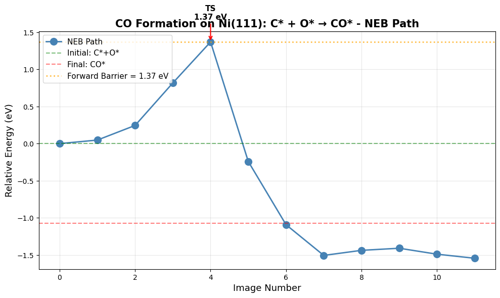
Creating NEB path animation...
   → Saved as neb_path.gif

   Visualizing initial state (C* + O*)...

   Visualizing transition state...

   Visualizing final state (CO*)...

✓ NEB analysis complete!
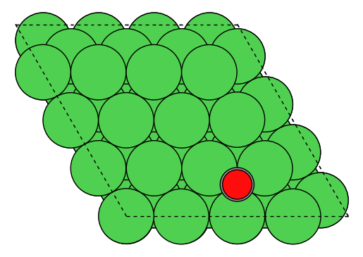
Missing UMA access?
Don’t have access to UMA yet? You can still explore this calculation!
Download example CO on Ni(111) structure and Download C+O on Ni(111) structure to test in the UMA demo (no login required) and explore the reaction pathway.
Comparison with Paper (Tables 4 & 5)
Expected Results from Paper:
Reaction Energy (C + O → CO*)**: -142.7 kJ/mol = -1.48 eV (exothermic, DFT-D3)
Activation Barrier (C + O → CO*)**: 153 kJ/mol = 1.59 eV (reverse/dissociation, DFT-D3)
CO Adsorption Energy: 1.82 eV = 175.6 kJ/mol (DFT-D3)
Reaction Direction:
Paper reports CO dissociation barrier (CO* → C* + O*), which is the reverse of the recombination we calculate
Forward (C* + O* → CO*): barrier = reverse_barrier - |ΔE| ≈ 1.59 - 1.48 ≈ 0.11 eV (very fast)
Reverse (CO* → C* + O*): barrier = 1.59 eV (very slow, kinetic bottleneck)
What to Check:
Reaction energy (C*+O* → CO*) should be strongly exothermic (~-1.5 eV)
Reverse barrier (CO dissociation) should be substantial (~1.6 eV)
Forward barrier (recombination) should be very small (~0.1 eV)
CO binds much more strongly than H (1.82 eV vs 0.60 eV)
Typical Variations:
Reaction energies typically accurate within 0.1-0.2 eV
Barriers more sensitive: expect ±0.2-0.3 eV variation
ZPE corrections typically add 0.05-0.15 eV to reaction energies
NEB convergence affects barrier more than reaction energy
Physical Insight:
Large reverse barrier (1.59 eV) makes CO dissociation very slow at low T
Small forward barrier (0.11 eV) means C+O rapidly recombine to CO
This explains why Ni produces CO in Fischer-Tropsch rather than keeping C and O separate
High temperatures needed to overcome the dissociation barrier for further C-C coupling
NEB Method Explained
The Nudged Elastic Band (NEB) method finds the minimum energy path between reactants and products:
Interpolate between initial and final states (5-9 images typical)
Add spring forces along the chain to maintain spacing
Project out spring components perpendicular to the path
Climbing image variant: highest energy image climbs to saddle point
Advantages:
No prior knowledge of transition state needed
Finds entire reaction coordinate
Robust for complex reactions
Limitations:
Computationally expensive (optimize N images)
May find wrong path if initial interpolation is poor
Explore on Your Own#
Image convergence: Run with 7 or 9 images. Does the barrier change?
Spring constant: Modify the NEB spring constant. How does this affect convergence?
Alternative paths: Try different initial CO/final C+O configurations. Are there multiple pathways?
Reverse barrier: Calculate E_a(reverse) = E_a(forward) - ΔE. Check Brønsted-Evans-Polanyi relationship.
Diffusion barriers: Compute NEB for C or O diffusion on the surface. How do they compare?
Summary and Best Practices#
Key Takeaways#
ML Potentials: UMa-S-1P1 provides ~1000× speedup over DFT with reasonable accuracy
Bulk optimization: Always use the ML-optimized lattice constant for consistency
Surface energies: Linear extrapolation eliminates finite-size effects
Adsorption: Test multiple sites; lowest energy may not be intuitive
Coverage: Lateral interactions become significant above ~0.3 ML
Barriers: NEB requires careful setup but yields full reaction pathway
Recommended Workflow for New Systems#
        graph TD
    A[Optimize Bulk] --> B[Calculate Surface Energies]
    B --> C[Wulff Construction]
    C --> D[Low-Coverage Adsorption]
    D --> E{Coverage Important?}
    E -->|Yes| F[Coverage Study]
    E -->|No| G[Reaction Barriers]
    F --> G
    G --> H[Microkinetic Modeling]
Accuracy Considerations#
Property |
Typical Error |
When Critical |
|---|---|---|
Lattice constants |
1-2% |
Strain effects, alloys |
Surface energies |
10-20% |
Nanoparticle shapes |
Adsorption energies |
0.1-0.3 eV |
Thermochemistry |
Barriers |
0.2-0.5 eV |
Kinetics, selectivity |
Rule of thumb: Use ML for screening → DFT for validation → Experiment for verification
Further Reading#
UMA Paper: Wood et al. 2025
OMat24 Paper: Barroso-Luque et al., 2024
OC20 Dataset: Chanussot et al., ACS Catalysis, 2021
ASE Tutorial: https://wiki.fysik.dtu.dk/ase/
Appendix: Troubleshooting#
Common Issues#
Problem: Convergence failures
Solution: Reduce
fmaxto 0.1 initially, tighten laterCheck if system is metastable (try different starting geometry)
Problem: NEB fails to find transition state
Solution: Use more images (9-11) or better initial guess
Try fixed-end NEB first, then climbing image
Problem: Unexpected adsorption energies
Solution: Visualize structures - check for distortions
Compare with multiple sites
Add D3 corrections
Problem: Out of memory
Solution: Reduce system size (smaller supercells)
Use fewer NEB images
Run on HPC with more RAM
Performance Tips#
Use batching: Relax multiple configurations in parallel
Start with DEBUG_MAX_STEPS=50: Get quick results, refine later
Cache bulk energies: Don’t recalculate reference systems
Trajectory analysis: Monitor optimization progress with ASE GUI
Caveats and Pitfalls#
Important Considerations
When using ML potentials for surface catalysis, be aware of these critical issues!
1. Task Selection: OMAT vs OC20#
Critical choice: Which task_name to use?
task_name="omat": Optimized for bulk and clean surface calculationsUse for: Part 1 (bulk), Part 2 (surface energies), Part 3 (Wulff)
Better for structural relaxations without adsorbates
task_name="oc20": Optimized for surface chemistry with adsorbatesUse for: Part 4-6 (all adsorbate calculations)
Trained on Open Catalyst data with adsorbate-surface interactions
Impact: Using wrong task can lead to 0.1-0.3 eV errors in adsorption energies!
2. D3 Dispersion Corrections#
Multiple decisions required:
Whether to use D3 at all?
Small adsorbates (H, O, N): D3 effect ~0.01-0.05 eV (often negligible)
Large molecules (CO, CO₂, aromatics): D3 effect ~0.1-0.3 eV (important!)
Physisorption: D3 critical (can change binding from repulsive to attractive)
RPBE was originally fit for chemisorption energies without D3 corrections, so adding D3 corrections may actually cause small adsorbates to overbind. However, it probably would be important for larger molecules. It’s relatively uncommon to see RPBE+D3 as a choice in the catalysis literature (compared to PBE+D3, or RPBE, or BEEF-vdW).
Which DFT functional for D3?
This tutorial uses
method="PBE"consistently for the D3 correction. This is often implied when papers say they use a D3 correction, but the results can be different if use the RPBE parameterizations.Original paper used PBE for bulk/surfaces, RPBE for adsorption. It’s not specified what D3 parameterization they used, but it’s likely PBE.
When to apply D3?
End-point correction (used here): Fast, run ML optimization then add D3 energy
During optimization: Slower but more accurate geometries
Impact: Usually <0.05 eV difference, but can be larger for weak interactions
3. Coverage Dependence Challenges#
Non-linearity at high coverage:
This tutorial assumes linear E_ads(θ) = E₀ + βθ
Reality: Often non-linear, especially near θ = 1 ML. See the plots generated - there is a linear regime for relatively high coverage, and relatively low coverage, but it’s not uniformly linear everywhere. As long as you consistently in one regime or the other a linear assumption is probably ok, but you could get into problems if solving microkinetic models where the coverage of the species in question changes significantly from very low to high.
Why: Phase transitions, adsorbate ordering, surface reconstruction
Solution: Test polynomial fits, look for ordering in visualizations
Low coverage limit:
At θ < 0.1 ML, coverage effects are tiny (<0.01 eV)
Hard to distinguish from numerical noise
Best practice: Focus on 0.25-1.0 ML range for fitting
4. Periodic Boundary Conditions#
UMa requires PBC=True in all directions!
atoms.set_pbc([True, True, True]) # Always required
Forgetting this causes crashes or wrong energies
Even for “gas phase” molecules in vacuum
5. Gas Phase Reference Energies#
Tricky cases:
H₂(g): UMa handles well (used in this tutorial)
H(g): May not be reliable (use H₂/2 instead)
CO(g), O₂(g): Usually okay, but check against DFT
Radicals: Often problematic
Best practice: Always use stable molecules as references (H₂, not H; H₂O, not OH)
6. Spin Polarization#
Key limitation: OC20/UMa does not include spin!
Paper used spin-polarized DFT
Impact: Usually small (0.05-0.1 eV)
Larger for:
Magnetic metals (Fe, Co, Ni)
Open-shell adsorbates (O*, OH*)
Reaction barriers with radicals
7. Constraint Philosophy#
Clean slabs (Part 2): No constraints (both surfaces relax)
Best for surface energy calculations
More physical for symmetric slabs
Adsorbate slabs (Part 4-6): Bottom layers fixed
Faster convergence
Prevents adsorbate-induced reconstruction
Standard practice in surface chemistry
Fairchem helper functions: Automatically apply sensible constraints
Trust their heuristics unless you have good reason not to
Check
atoms.constraintsto see what was applied
8. Complex Surface Structures#
This tutorial uses low-index facets (111, 100, 110, 211)
Well-defined, symmetric
Easy to generate and analyze
Real catalysts have:
Steps, kinks, grain boundaries
Support interfaces
Defects and vacancies
Challenge: Harder to generate, more configurations to test
9. Slab Thickness and Vacuum#
Convergence tests critical but expensive:
This tutorial uses “reasonable” values (4-8 layers, 10 Å vacuum)
Always check convergence for new systems
Especially important for:
Metals with long electron screening (Au, Ag)
Charged adsorbates
Strong adsorbate-induced reconstruction
10. NEB Convergence#
Most computationally expensive part:
May need 7-11 images (not just 5)
Initial guess matters a lot
Can get stuck in local minima
Tricks:
Use dimer method to find better TS guess (as shown in Part 6)
Start with coarse convergence (fmax=0.2), refine later
Visualize the path - does it make chemical sense?
Try different spring constants (0.1-1.0 eV/Å)
11. Lattice Constant Source#
Consistency is key:
Use ML-optimized lattice constant throughout (as done here)
Don’t mix: ML lattice + DFT surface energies = inconsistent
Alternative: Use experimental lattice constant for everything
12. Adsorbate Placement#
Multiple local minima:
Surface chemistry is not convex!
Always test multiple adsorption sites
Fairchem helpers generate ~5 configurations in this tutorial, but you may need more to search many modes. You can already try methods like minima hopping or other global optimization methods to sample more configurations.
For complex adsorbates:
Test different orientations
May need 10-20 configurations
Consider genetic algorithms or basin hopping
Congratulations! 🎉
You’ve completed a comprehensive computational catalysis workflow using state-of-the-art ML potentials. You can now:
Characterize catalyst surfaces computationally
Predict nanoparticle shapes
Calculate reaction thermodynamics and kinetics
Apply these methods to your own research questions
Next steps:
Apply to your catalyst system of interest
Validate key results with DFT
Develop microkinetic models
Publish your findings!